BIOS_sctransform-normalisation
Ruqian Lyu
11/30/2020
Last updated: 2020-11-30
Checks: 6 1
Knit directory: bios_2020_single-cell-workshop-svi/
This reproducible R Markdown analysis was created with workflowr (version 1.6.2). The Checks tab describes the reproducibility checks that were applied when the results were created. The Past versions tab lists the development history.
The R Markdown file has unstaged changes. To know which version of the R Markdown file created these results, you’ll want to first commit it to the Git repo. If you’re still working on the analysis, you can ignore this warning. When you’re finished, you can run wflow_publish to commit the R Markdown file and build the HTML.
Great job! The global environment was empty. Objects defined in the global environment can affect the analysis in your R Markdown file in unknown ways. For reproduciblity it’s best to always run the code in an empty environment.
The command set.seed(20190102) was run prior to running the code in the R Markdown file. Setting a seed ensures that any results that rely on randomness, e.g. subsampling or permutations, are reproducible.
Great job! Recording the operating system, R version, and package versions is critical for reproducibility.
Nice! There were no cached chunks for this analysis, so you can be confident that you successfully produced the results during this run.
Great job! Using relative paths to the files within your workflowr project makes it easier to run your code on other machines.
Great! You are using Git for version control. Tracking code development and connecting the code version to the results is critical for reproducibility.
The results in this page were generated with repository version b0c7d78. See the Past versions tab to see a history of the changes made to the R Markdown and HTML files.
Note that you need to be careful to ensure that all relevant files for the analysis have been committed to Git prior to generating the results (you can use wflow_publish or wflow_git_commit). workflowr only checks the R Markdown file, but you know if there are other scripts or data files that it depends on. Below is the status of the Git repository when the results were generated:
Ignored files:
    Ignored:    .Rhistory
    Ignored:    .Rproj.user/

Untracked files:
    Untracked:  .Renviron
    Untracked:  Rcode.R
    Untracked:  Rcode2.R
    Untracked:  Rplots.pdf
    Untracked:  analysis/about.Rmd
    Untracked:  analysis/license.Rmd
    Untracked:  data/
    Untracked:  memusage.txt
    Untracked:  raw_data/
    Untracked:  rscript.R
    Untracked:  untar_path/

Unstaged changes:
    Modified:   analysis/BIOS_analysis-workflow.Rmd
    Modified:   analysis/BIOS_dataset-source.Rmd
    Modified:   analysis/BIOS_sctransform-normalisation.Rmd
    Modified:   analysis/_site.yml
    Modified:   bios.bib
Note that any generated files, e.g. HTML, png, CSS, etc., are not included in this status report because it is ok for generated content to have uncommitted changes.
These are the previous versions of the repository in which changes were made to the R Markdown (analysis/BIOS_sctransform-normalisation.Rmd) and HTML (public/BIOS_sctransform-normalisation.html) files. If you’ve configured a remote Git repository (see ?wflow_git_remote), click on the hyperlinks in the table below to view the files as they were in that past version.
| File | Version | Author | Date | Message |
|---|---|---|---|---|
| Rmd | eab0b17 | rlyu | 2020-11-16 | finalising analysis workflow and sctransform |
| html | eab0b17 | rlyu | 2020-11-16 | finalising analysis workflow and sctransform |
| Rmd | 110616a | rlyu | 2020-11-12 | updat workflow, still need to do varying Ks |
| Rmd | 9bd198a | rlyu | 2020-11-12 | update analysis workflow |
| Rmd | 11c8318 | rlyu | 2020-11-12 | Adding more descriptions |
sctransform
Different from the size_factor-based normalisation method that we used before, sctransform is based on probabilistic models for normalisation and variance stablisation of UMI-count data from scRNAseq. Instead of using a constant factor for normalising all genes for one cell, sctransform (Hafemeister and Satija 2019) models and scales each gene individually.
sctransform fits a generalised linear model with a negative binomial error model for each gene with the sequencing depth (library size) as a covariate followed by a regularisation procedure to control overfitting. The residuals from the regularised regression model is then treated as normalised expression levels with variation caused by sequencing depth removed.
suppressPackageStartupMessages({
    library(sctransform)
    library(ggplot2)
    library(scater)
    library(scran)
  }
)
sce.pbmc <- readRDS(file = "raw_data/sce_pbmc.rds")
We use the log10_umi as the latent variable that will be regressed out in the normalised gene expression values.
set.seed(10000)

colData(sce.pbmc)$log10_umi <- log(colData(sce.pbmc)$total,base=10)
pbmc.sctrans <- suppressWarnings(sctransform::vst(assay(sce.pbmc,"counts"),
                                 cell_attr = colData(sce.pbmc),
                                 latent_var = "log10_umi", verbosity = FALSE))

## Warning related issue: https://github.com/ChristophH/sctransform/issues/25Add to assay field
pbmc.sctrans stores returned value from running variance stablisation using sctransform. The normalised values are stored in the matrix y. We now add y to the sce object in the assay field with asaay name “SCT”. This is equivalant to the logcounts assay.
Select highly variable genes
Feature selection after sctransform normalisation is straightforward. We can just select the top genes that have a high residual variance which contribute the most biological sources of variation.
          detection_rate gmean variance residual_mean residual_variance
IGKC                0.27  0.60   184.08          2.89            135.91
S100A8              0.62  2.15   633.20          3.75            125.33
S100A9              0.70  2.70   921.73          3.68            113.23
GNLY                0.24  0.45    74.24          2.05             96.29
LYZ                 0.65  2.82  1042.16          3.70             82.80
IGLC3               0.10  0.16   590.98          1.11             71.41
IGLC2               0.19  0.26 16209.67          1.16             69.35
NKG7                0.38  0.84    45.18          1.76             41.94
PPBP                0.03  0.05    10.27          0.55             41.88
PF4                 0.03  0.04     3.27          0.55             41.33
CCL5                0.35  0.85    38.41          1.70             32.14
SDPR                0.02  0.03     1.20          0.44             31.22
GNG11               0.04  0.04     1.01          0.43             30.53
HIST1H2AC           0.06  0.06     2.78          0.42             27.31
GZMB                0.10  0.14     9.18          0.62             27.26
TUBB1               0.02  0.03     1.27          0.39             27.14
CD74                0.92  6.11  1597.07          1.75             26.45
FTL                 0.99 12.79  1475.18          1.45             22.33
JCHAIN              0.07  0.09    12.44          0.40             21.84
S100A12             0.26  0.49    16.41          0.95             21.73
KLRB1               0.24  0.46    15.92          0.99             21.64
CST3                0.56  1.77   306.70          1.51             21.15
select 3,000 highly variable genes for downstream analysis
runPCA with HVGs
Next, we runPCA with the selected number of highly variable genes.
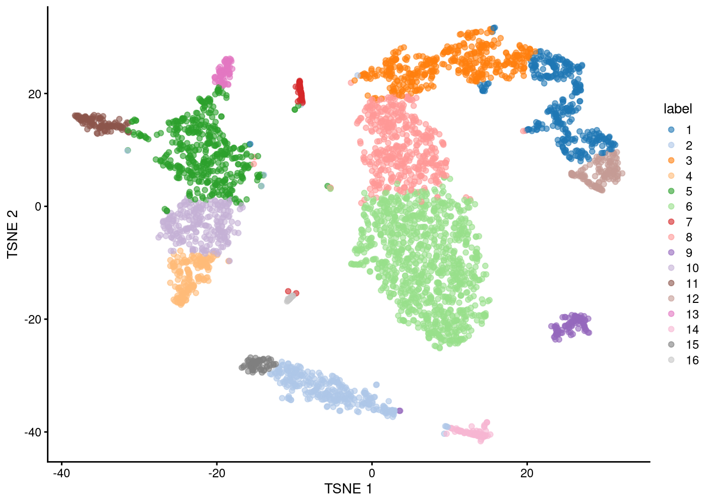
Generate TSNE plot using PCs
Clustering
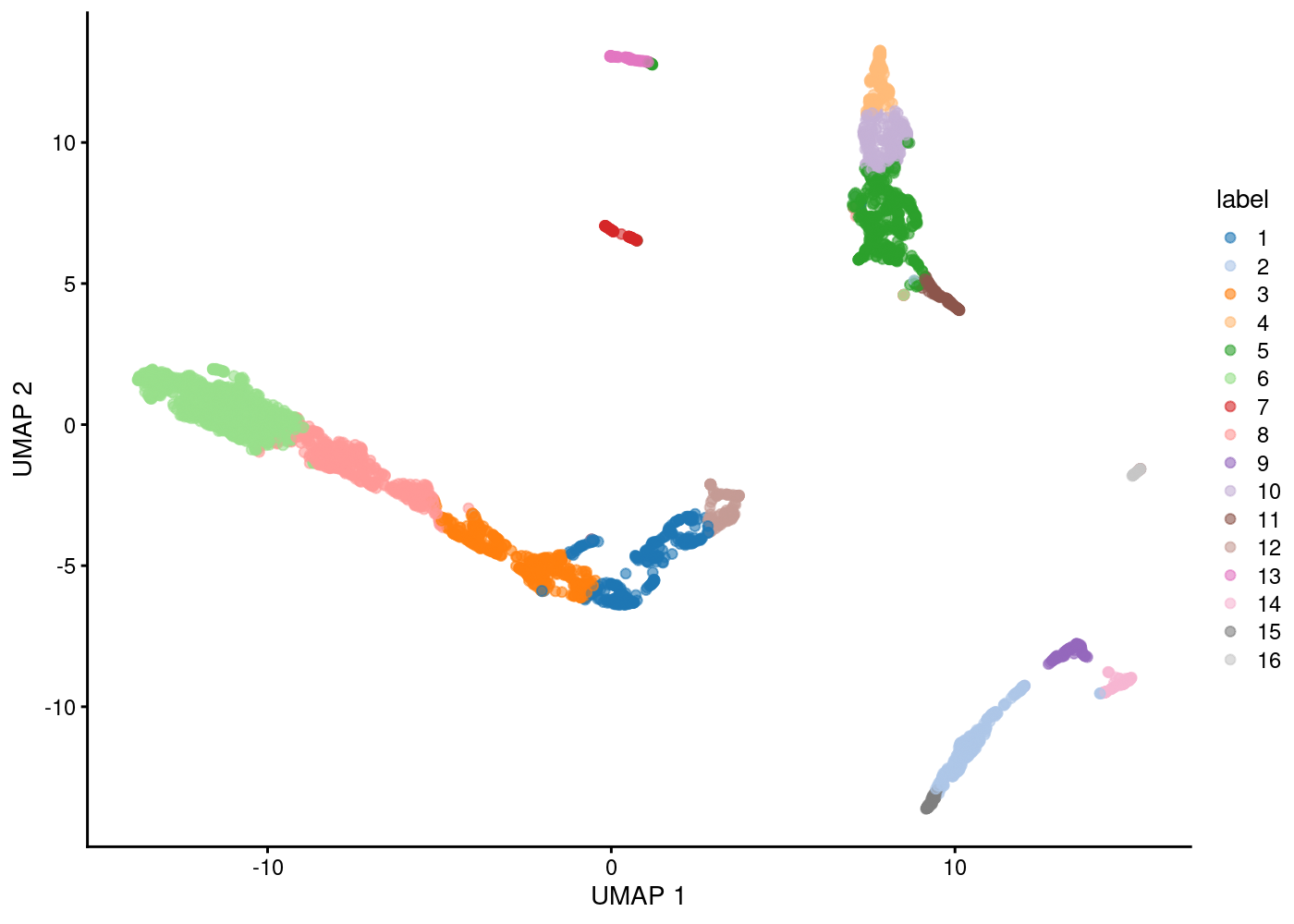
The remaining steps are similar to those presented in the main workflow.
Plot Clusters
| Version | Author | Date |
|---|---|---|
| eab0b17 | rlyu | 2020-11-16 |
| Version | Author | Date |
|---|---|---|
| eab0b17 | rlyu | 2020-11-16 |
plotExpression(sce.pbmc, features=c("CD14", "CD68",
    "MNDA", "FCGR3A"), x="label", colour_by="label",exprs_values = "SCT")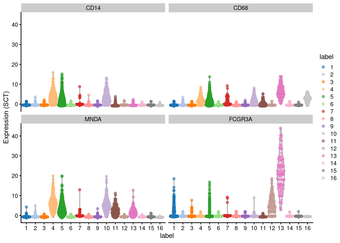
| Version | Author | Date |
|---|---|---|
| eab0b17 | rlyu | 2020-11-16 |
More info
sctransform is also integrated and interfaced with Seurat package which you can find more information here: https://satijalab.org/seurat/v3.2/sctransform_vignette.html
References
SessionInfo
R version 4.0.3 (2020-10-10)
Platform: x86_64-pc-linux-gnu (64-bit)
Running under: Red Hat Enterprise Linux

Matrix products: default
BLAS/LAPACK: /usr/lib64/libopenblasp-r0.3.3.so

locale:
 [1] LC_CTYPE=en_AU.UTF-8       LC_NUMERIC=C
 [3] LC_TIME=en_AU.UTF-8        LC_COLLATE=en_AU.UTF-8
 [5] LC_MONETARY=en_AU.UTF-8    LC_MESSAGES=en_AU.UTF-8
 [7] LC_PAPER=en_AU.UTF-8       LC_NAME=C
 [9] LC_ADDRESS=C               LC_TELEPHONE=C
[11] LC_MEASUREMENT=en_AU.UTF-8 LC_IDENTIFICATION=C

attached base packages:
[1] parallel  stats4    stats     graphics  grDevices utils     datasets
[8] methods   base

other attached packages:
 [1] scran_1.18.0                scater_1.18.0
 [3] SingleCellExperiment_1.12.0 SummarizedExperiment_1.20.0
 [5] Biobase_2.50.0              GenomicRanges_1.42.0
 [7] GenomeInfoDb_1.26.0         IRanges_2.24.0
 [9] S4Vectors_0.28.0            BiocGenerics_0.36.0
[11] MatrixGenerics_1.2.0        matrixStats_0.57.0
[13] ggplot2_3.3.2               sctransform_0.3.1

loaded via a namespace (and not attached):
 [1] bitops_1.0-6              fs_1.5.0
 [3] rprojroot_1.3-2           tools_4.0.3
 [5] backports_1.2.0           R6_2.5.0
 [7] irlba_2.3.3               vipor_0.4.5
 [9] uwot_0.1.8                colorspace_1.4-1
[11] withr_2.3.0               tidyselect_1.1.0
[13] gridExtra_2.3             compiler_4.0.3
[15] git2r_0.27.1              BiocNeighbors_1.8.0
[17] DelayedArray_0.16.0       labeling_0.4.2
[19] scales_1.1.1              stringr_1.4.0
[21] digest_0.6.27             rmarkdown_2.5
[23] XVector_0.30.0            pkgconfig_2.0.3
[25] htmltools_0.5.0           parallelly_1.21.0
[27] sparseMatrixStats_1.2.0   limma_3.46.0
[29] rlang_0.4.8               rstudioapi_0.11
[31] FNN_1.1.3                 DelayedMatrixStats_1.12.0
[33] farver_2.0.3              generics_0.1.0
[35] BiocParallel_1.24.0       dplyr_1.0.2
[37] RCurl_1.98-1.2            magrittr_1.5
[39] BiocSingular_1.6.0        GenomeInfoDbData_1.2.4
[41] scuttle_1.0.0             Matrix_1.2-18
[43] Rcpp_1.0.5                ggbeeswarm_0.6.0
[45] munsell_0.5.0             viridis_0.5.1
[47] lifecycle_0.2.0           stringi_1.5.3
[49] whisker_0.4               yaml_2.2.1
[51] edgeR_3.32.0              MASS_7.3-53
[53] zlibbioc_1.36.0           Rtsne_0.15
[55] plyr_1.8.6                grid_4.0.3
[57] listenv_0.8.0             promises_1.1.1
[59] dqrng_0.2.1               crayon_1.3.4
[61] lattice_0.20-41           cowplot_1.1.0
[63] beachmat_2.6.0            locfit_1.5-9.4
[65] knitr_1.30                pillar_1.4.6
[67] igraph_1.2.6              future.apply_1.6.0
[69] reshape2_1.4.4            codetools_0.2-16
[71] glue_1.4.2                evaluate_0.14
[73] vctrs_0.3.4               httpuv_1.5.4
[75] gtable_0.3.0              purrr_0.3.4
[77] future_1.20.1             xfun_0.19
[79] rsvd_1.0.3                RSpectra_0.16-0
[81] later_1.1.0.1             viridisLite_0.3.0
[83] tibble_3.0.4              beeswarm_0.2.3
[85] workflowr_1.6.2           statmod_1.4.35
[87] bluster_1.0.0             globals_0.13.1
[89] ellipsis_0.3.1
Hafemeister, Christoph, and Rahul Satija. 2019. “Normalization and Variance Stabilization of Single-Cell RNA-seq Data Using Regularized Negative Binomial Regression.” Genome Biol. 20 (1): 296.
─ Session info ───────────────────────────────────────────────────────────────
 setting  value
 version  R version 4.0.3 (2020-10-10)
 os       Red Hat Enterprise Linux
 system   x86_64, linux-gnu
 ui       X11
 language (EN)
 collate  en_AU.UTF-8
 ctype    en_AU.UTF-8
 tz       Australia/Melbourne
 date     2020-11-30

─ Packages ───────────────────────────────────────────────────────────────────
 package              * version  date       lib source
 assertthat             0.2.1    2019-03-21 [1] CRAN (R 4.0.2)
 backports              1.2.0    2020-11-02 [1] CRAN (R 4.0.2)
 beachmat               2.6.0    2020-10-27 [1] Bioconductor
 beeswarm               0.2.3    2016-04-25 [1] CRAN (R 4.0.2)
 Biobase              * 2.50.0   2020-10-27 [1] Bioconductor
 BiocGenerics         * 0.36.0   2020-10-27 [1] Bioconductor
 BiocNeighbors          1.8.0    2020-10-27 [1] Bioconductor
 BiocParallel           1.24.0   2020-10-27 [1] Bioconductor
 BiocSingular           1.6.0    2020-10-27 [1] Bioconductor
 bitops                 1.0-6    2013-08-17 [1] CRAN (R 4.0.2)
 bluster                1.0.0    2020-10-27 [1] Bioconductor
 callr                  3.5.1    2020-10-13 [1] CRAN (R 4.0.2)
 cli                    2.1.0    2020-10-12 [1] CRAN (R 4.0.2)
 codetools              0.2-16   2018-12-24 [2] CRAN (R 4.0.3)
 colorspace             1.4-1    2019-03-18 [1] CRAN (R 4.0.2)
 cowplot                1.1.0    2020-09-08 [1] CRAN (R 4.0.2)
 crayon                 1.3.4    2017-09-16 [1] CRAN (R 4.0.2)
 DelayedArray           0.16.0   2020-10-27 [1] Bioconductor
 DelayedMatrixStats     1.12.0   2020-10-27 [1] Bioconductor
 desc                   1.2.0    2018-05-01 [1] CRAN (R 4.0.2)
 devtools               2.3.2    2020-09-18 [1] CRAN (R 4.0.2)
 digest                 0.6.27   2020-10-24 [1] CRAN (R 4.0.2)
 dplyr                  1.0.2    2020-08-18 [1] CRAN (R 4.0.2)
 dqrng                  0.2.1    2019-05-17 [1] CRAN (R 4.0.2)
 edgeR                  3.32.0   2020-10-27 [1] Bioconductor
 ellipsis               0.3.1    2020-05-15 [1] CRAN (R 4.0.2)
 evaluate               0.14     2019-05-28 [1] CRAN (R 4.0.2)
 fansi                  0.4.1    2020-01-08 [1] CRAN (R 4.0.2)
 farver                 2.0.3    2020-01-16 [1] CRAN (R 4.0.2)
 FNN                    1.1.3    2019-02-15 [1] CRAN (R 4.0.2)
 fs                     1.5.0    2020-07-31 [1] CRAN (R 4.0.2)
 future                 1.20.1   2020-11-03 [1] CRAN (R 4.0.2)
 future.apply           1.6.0    2020-07-01 [1] CRAN (R 4.0.2)
 generics               0.1.0    2020-10-31 [1] CRAN (R 4.0.2)
 GenomeInfoDb         * 1.26.0   2020-10-27 [1] Bioconductor
 GenomeInfoDbData       1.2.4    2020-11-04 [1] Bioconductor
 GenomicRanges        * 1.42.0   2020-10-27 [1] Bioconductor
 ggbeeswarm             0.6.0    2017-08-07 [1] CRAN (R 4.0.2)
 ggplot2              * 3.3.2    2020-06-19 [1] CRAN (R 4.0.2)
 git2r                  0.27.1   2020-05-03 [1] CRAN (R 4.0.2)
 globals                0.13.1   2020-10-11 [1] CRAN (R 4.0.2)
 glue                   1.4.2    2020-08-27 [1] CRAN (R 4.0.2)
 gridExtra              2.3      2017-09-09 [1] CRAN (R 4.0.2)
 gtable                 0.3.0    2019-03-25 [1] CRAN (R 4.0.2)
 htmltools              0.5.0    2020-06-16 [1] CRAN (R 4.0.2)
 httpuv                 1.5.4    2020-06-06 [1] CRAN (R 4.0.2)
 igraph                 1.2.6    2020-10-06 [1] CRAN (R 4.0.2)
 IRanges              * 2.24.0   2020-10-27 [1] Bioconductor
 irlba                  2.3.3    2019-02-05 [1] CRAN (R 4.0.2)
 knitr                  1.30     2020-09-22 [1] CRAN (R 4.0.2)
 labeling               0.4.2    2020-10-20 [1] CRAN (R 4.0.2)
 later                  1.1.0.1  2020-06-05 [1] CRAN (R 4.0.2)
 lattice                0.20-41  2020-04-02 [2] CRAN (R 4.0.3)
 lifecycle              0.2.0    2020-03-06 [1] CRAN (R 4.0.2)
 limma                  3.46.0   2020-10-27 [1] Bioconductor
 listenv                0.8.0    2019-12-05 [1] CRAN (R 4.0.2)
 locfit                 1.5-9.4  2020-03-25 [1] CRAN (R 4.0.2)
 magrittr               1.5      2014-11-22 [1] CRAN (R 4.0.2)
 MASS                   7.3-53   2020-09-09 [2] CRAN (R 4.0.3)
 Matrix                 1.2-18   2019-11-27 [2] CRAN (R 4.0.3)
 MatrixGenerics       * 1.2.0    2020-10-27 [1] Bioconductor
 matrixStats          * 0.57.0   2020-09-25 [1] CRAN (R 4.0.2)
 memoise                1.1.0    2017-04-21 [1] CRAN (R 4.0.2)
 munsell                0.5.0    2018-06-12 [1] CRAN (R 4.0.2)
 parallelly             1.21.0   2020-10-27 [1] CRAN (R 4.0.2)
 pillar                 1.4.6    2020-07-10 [1] CRAN (R 4.0.2)
 pkgbuild               1.1.0    2020-07-13 [1] CRAN (R 4.0.2)
 pkgconfig              2.0.3    2019-09-22 [1] CRAN (R 4.0.2)
 pkgload                1.1.0    2020-05-29 [1] CRAN (R 4.0.2)
 plyr                   1.8.6    2020-03-03 [1] CRAN (R 4.0.2)
 prettyunits            1.1.1    2020-01-24 [1] CRAN (R 4.0.2)
 processx               3.4.4    2020-09-03 [1] CRAN (R 4.0.2)
 promises               1.1.1    2020-06-09 [1] CRAN (R 4.0.2)
 ps                     1.4.0    2020-10-07 [1] CRAN (R 4.0.2)
 purrr                  0.3.4    2020-04-17 [1] CRAN (R 4.0.2)
 R6                     2.5.0    2020-10-28 [1] CRAN (R 4.0.2)
 Rcpp                   1.0.5    2020-07-06 [1] CRAN (R 4.0.2)
 RCurl                  1.98-1.2 2020-04-18 [1] CRAN (R 4.0.2)
 remotes                2.2.0    2020-07-21 [1] CRAN (R 4.0.2)
 reshape2               1.4.4    2020-04-09 [1] CRAN (R 4.0.2)
 rlang                  0.4.8    2020-10-08 [1] CRAN (R 4.0.2)
 rmarkdown              2.5      2020-10-21 [1] CRAN (R 4.0.2)
 rprojroot              1.3-2    2018-01-03 [1] CRAN (R 4.0.2)
 RSpectra               0.16-0   2019-12-01 [1] CRAN (R 4.0.2)
 rstudioapi             0.11     2020-02-07 [1] CRAN (R 4.0.2)
 rsvd                   1.0.3    2020-02-17 [1] CRAN (R 4.0.2)
 Rtsne                  0.15     2018-11-10 [1] CRAN (R 4.0.2)
 S4Vectors            * 0.28.0   2020-10-27 [1] Bioconductor
 scales                 1.1.1    2020-05-11 [1] CRAN (R 4.0.2)
 scater               * 1.18.0   2020-10-27 [1] Bioconductor
 scran                * 1.18.0   2020-10-27 [1] Bioconductor
 sctransform          * 0.3.1    2020-10-08 [1] CRAN (R 4.0.2)
 scuttle                1.0.0    2020-10-27 [1] Bioconductor
 sessioninfo            1.1.1    2018-11-05 [1] CRAN (R 4.0.2)
 SingleCellExperiment * 1.12.0   2020-10-27 [1] Bioconductor
 sparseMatrixStats      1.2.0    2020-10-27 [1] Bioconductor
 statmod                1.4.35   2020-10-19 [1] CRAN (R 4.0.2)
 stringi                1.5.3    2020-09-09 [1] CRAN (R 4.0.2)
 stringr                1.4.0    2019-02-10 [1] CRAN (R 4.0.2)
 SummarizedExperiment * 1.20.0   2020-10-27 [1] Bioconductor
 testthat               3.0.0    2020-10-31 [1] CRAN (R 4.0.2)
 tibble                 3.0.4    2020-10-12 [1] CRAN (R 4.0.2)
 tidyselect             1.1.0    2020-05-11 [1] CRAN (R 4.0.2)
 usethis                1.6.3    2020-09-17 [1] CRAN (R 4.0.2)
 uwot                   0.1.8    2020-03-16 [1] CRAN (R 4.0.2)
 vctrs                  0.3.4    2020-08-29 [1] CRAN (R 4.0.2)
 vipor                  0.4.5    2017-03-22 [1] CRAN (R 4.0.2)
 viridis                0.5.1    2018-03-29 [1] CRAN (R 4.0.2)
 viridisLite            0.3.0    2018-02-01 [1] CRAN (R 4.0.2)
 whisker                0.4      2019-08-28 [1] CRAN (R 4.0.2)
 withr                  2.3.0    2020-09-22 [1] CRAN (R 4.0.2)
 workflowr              1.6.2    2020-04-30 [1] CRAN (R 4.0.2)
 xfun                   0.19     2020-10-30 [1] CRAN (R 4.0.2)
 XVector                0.30.0   2020-10-27 [1] Bioconductor
 yaml                   2.2.1    2020-02-01 [1] CRAN (R 4.0.2)
 zlibbioc               1.36.0   2020-10-27 [1] Bioconductor

[1] /mnt/mcscratch/rlyu/Software/R/4.0/library
[2] /opt/R/4.0.3/lib/R/library