2024-08-13_hyperparameters
Ruqian Lyu
2024-08-13
Last updated: 2024-08-20
Checks: 6 1
Knit directory:
ieny_2024_spatial-rna-graphs/
This reproducible R Markdown analysis was created with workflowr (version 1.7.0). The Checks tab describes the reproducibility checks that were applied when the results were created. The Past versions tab lists the development history.
Great! Since the R Markdown file has been committed to the Git repository, you know the exact version of the code that produced these results.
Great job! The global environment was empty. Objects defined in the global environment can affect the analysis in your R Markdown file in unknown ways. For reproduciblity it’s best to always run the code in an empty environment.
The command set.seed(20240820) was run prior to running
the code in the R Markdown file. Setting a seed ensures that any results
that rely on randomness, e.g. subsampling or permutations, are
reproducible.
Great job! Recording the operating system, R version, and package versions is critical for reproducibility.
Nice! There were no cached chunks for this analysis, so you can be confident that you successfully produced the results during this run.
Using absolute paths to the files within your workflowr project makes it difficult for you and others to run your code on a different machine. Change the absolute path(s) below to the suggested relative path(s) to make your code more reproducible.
| absolute | relative |
|---|---|
| /mnt/beegfs/mccarthy/backed_up/general/rlyu/Projects/ieny_2024_spatial-rna-graphs | . |
Great! You are using Git for version control. Tracking code development and connecting the code version to the results is critical for reproducibility.
The results in this page were generated with repository version 81c14c9. See the Past versions tab to see a history of the changes made to the R Markdown and HTML files.
Note that you need to be careful to ensure that all relevant files for
the analysis have been committed to Git prior to generating the results
(you can use wflow_publish or
wflow_git_commit). workflowr only checks the R Markdown
file, but you know if there are other scripts or data files that it
depends on. Below is the status of the Git repository when the results
were generated:
Ignored files:
    Ignored:    .Rproj.user/

Untracked files:
    Untracked:  .Renviron
    Untracked:  .gitignore
    Untracked:  .gitlab-ci.yml
    Untracked:  _workflowr.yml
    Untracked:  analysis/
    Untracked:  code/
    Untracked:  data/
    Untracked:  envs/install-packages.md
    Untracked:  figures/
    Untracked:  gen_sim/dense1/
    Untracked:  gen_sim/dense2/
    Untracked:  gen_sim/dense4/
    Untracked:  gen_sim/simulated/data/analysis/
    Untracked:  gen_sim/simulated/data/batched.matrix.tsv.gz
    Untracked:  gen_sim/simulated/data/cell_info.tsv.gz
    Untracked:  gen_sim/simulated/data/coordinate_minmax.tsv
    Untracked:  gen_sim/simulated/data/feature.tsv.gz
    Untracked:  gen_sim/simulated/data/hexagon.d_12.s_2.tsv.gz
    Untracked:  gen_sim/simulated/data/matrix.csv
    Untracked:  gen_sim/simulated/data/matrix.tsv.gz
    Untracked:  gen_sim/simulated/data/model.rgb.tsv
    Untracked:  gen_sim/simulated/data/model.true.tsv.gz
    Untracked:  gen_sim/simulated/data/pixel_label.uniq.tsv.gz
    Untracked:  gen_sim/simulated/data/processed/
    Untracked:  gen_sim/simulated/data/raw/
    Untracked:  gen_sim/simulated/data/subgraph/
    Untracked:  gen_sim/simulated/emb_models/
    Untracked:  gen_sim/simulated/embs.npy
    Untracked:  gen_sim/simulated/embs_pytorchversion.npy
    Untracked:  gen_sim/simulated/embs_pytorchversion_dmax1.npy
    Untracked:  gen_sim/simulated_rec/
    Untracked:  ieny_2024_spatial-rna-graphs.Rproj
    Untracked:  output/
    Untracked:  requirements.txt
    Untracked:  tutorial_notebooks/.ipynb_checkpoints/
    Untracked:  tutorial_notebooks/03_2_expl_integration_multiple_samples_increase_r.ipynb
    Untracked:  tutorial_notebooks/04_expl_model_hyper_parameters.ipynb
    Untracked:  tutorial_notebooks/check_gat.ipynb
    Untracked:  tutorial_notebooks/check_mem_usage.ipynb
    Untracked:  tutorial_notebooks/clustering_analysis.ipynb
    Untracked:  tutorial_notebooks/demo_overfit.ipynb
    Untracked:  tutorial_notebooks/expl_grad_multi_scale.ipynb
    Untracked:  tutorial_notebooks/expl_simulated_data_pytorch_versions_experimen.ipynb
    Untracked:  tutorial_notebooks/reproduciable_expl_simulated_data_pytorch_versions.ipynb
    Untracked:  tutorial_notebooks/stopping_cri.ipynb
    Untracked:  tutorial_notebooks/test_SpatialRNA.ipynb
    Untracked:  tutorial_notebooks/test_SpatialRNA_large_radius.ipynb
    Untracked:  tutorial_notebooks/test_batch_from_data_list.ipynb
    Untracked:  tutorial_notebooks/test_remote_backend.ipynb
    Untracked:  workflows/

Unstaged changes:
    Modified:   envs/environment.yml
    Modified:   tutorial_notebooks/01_expl_simulated_data_pytorch_versions.ipynb
    Deleted:    tutorial_notebooks/03_2_expl_integration_multiple_sample_increase_r.ipynb
Note that any generated files, e.g. HTML, png, CSS, etc., are not included in this status report because it is ok for generated content to have uncommitted changes.
There are no past versions. Publish this analysis with
wflow_publish() to start tracking its development.
#.libPaths()
#setwd("/mnt/beegfs/mccarthy/backed_up/general/rlyu/Projects/ieny_2024_spatial-rna-graphs")
.libPaths( "/mnt/beegfs/mccarthy/backed_up/general/rlyu/Software/Rlibs/4.1.2")
suppressPackageStartupMessages({
  library(readr)
  library(ggplot2)
  library(plotly)
  library(dplyr)
})
#getwd()
Ground-truth simulation labels
groundtrue_labels <- read.table("gen_sim/simulated/data/pixel_label.uniq.tsv.gz",
                                sep = "\t",
                                header = 1)

groundtruth_color <- read.table("gen_sim/simulated/data/model.rgb.tsv",
                                sep = "\t",header=1)
groundtruth_hex <- rgb(groundtruth_color[,c("R","G","B")])
names(groundtruth_hex) <- groundtruth_color$cell_label

head(groundtrue_labels)
X Y cell_id cell_label cell_shape
1 0 31.39 98 fibroblast rod
2 0 345.69 758 fibroblast rod
3 0 278.56 626 fibroblast rod
4 0 317.52 692 fibroblast diamond
5 0 372.04 792 fibroblast diamond
6 0 125.38 231 fibroblast backgroundgroundtrue_labels %>%
ggplot()+geom_point(mapping = aes(
x=X,y=Y,
color = cell_label
),size=0.01,alpha=0.8)+
scale_color_manual(values = groundtruth_hex)+
theme_minimal(base_size = 15)+
theme(panel.grid = element_blank(),
axis.ticks = element_blank(),
axis.text = element_blank(),
legend.position = "None")+coord_equal()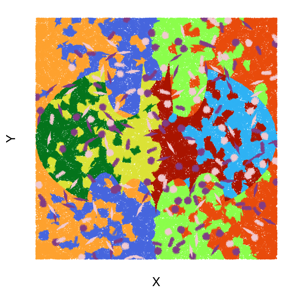
Effects of radius size, and numbers of edge_label_index
used for training
The simulated dataset with ground-truth labels is very helpful for
assessing the impact of different hyper-paramters in our GNN models. As
a starting point, we first assess the effects of different radius
values, and how it compares among using different numbers of
edge_label_index for model training.
Note in tutorial 01, we explained that when training the model, we randomly sampled 50,000 edges in the graph and supplied them as positive node pairs through the
edge_label_indexargument in the loader function.Intuitively, one may expect that the training results will be more stable when more edges are used for training.
In the following set of analyses, we evaluate the training results through comparing the clustering labels (through kmeans clustering) obtained from each training setting with the ground-truth cell labels. We repeat each training setting 5 times.
We adopt an early-stopping strategy for GNN training, in which we set the maximum number of epochs to be 50, with patience 10 based on the training loss. It means we stop the training when we do not see loss improvement in 10 epochs regardless of reaching the maximum epoch number or not.
To mitigate the effect of clustering algorithms performance, we use three k values (10,11,12) when clustering transcripts embeddings obtained from each training setting, and measure the consistency of clustering labels with the 10 ground-truth cell type labels using adjusted rand index (ARI). Finally, we only show the largest ARI value out of the three k values for each repeat of each training setting.
all_res <- list.files("output/test_radius",
                      pattern = "ari_r.*.csv",
                      recursive = TRUE,full.names = T)
all_res <- all_res[!grepl("increase_epoch",all_res)]
#length(all_res)

acc_results <- lapply(all_res,
       function(file_name){
         nedges = strsplit(file_name,"/")[[1]][3]
         radius = strsplit(file_name,"/")[[1]][5]
         rep = strsplit(file_name,"/")[[1]][4]
         acc_res = read.csv(file_name,header = 1,col.names = c("id","ari"))
         acc_res$nedges = nedges
         acc_res$rep <- rep

         acc_res$radius = radius
         acc_res[1:3,"id"] <- paste0("all_",acc_res[1:3,"id"])
         acc_res[4:6,"id"] <- paste0("cell_",acc_res[4:6,"id"])
         acc_res$type = c("all","all","all","cell","cell","cell")
         acc_res
       })

acc_results_edge_effect_df <- do.call(rbind,acc_results)
acc_results_edge_effect_df$nedges <- as.numeric(gsub("nedges","",
                                                     acc_results_edge_effect_df$nedges))

acc_results_edge_effect_df$radius <- gsub("ari_","",
                                          acc_results_edge_effect_df$radius)
acc_results_edge_effect_df$radius <- gsub(".csv","",
                                          acc_results_edge_effect_df$radius)


#
# all_res <- all_res[!grepl("r0.5",all_res)]
# length(all_res)
The type group factor indicates whether the ARI score
has been calculated using all transcripts or only transcripts in cell
boundaries.
p1 <- acc_results_edge_effect_df %>%
    group_by(type,radius,nedges,rep) %>%
  arrange(-ari) %>%
  slice(1) %>%
  ggplot()+
  geom_boxplot(mapping = aes(x = "type", y = ari,fill=type),
               outlier.shape = 12)+
  geom_jitter(mapping = aes(x = "type", y = ari),height = 0,
              size=0.1)+
  facet_grid(cols = vars(nedges),rows = vars(radius),
             scales = "free_x",
             space="free_x")+
  theme_bw(base_size = 10)+
  theme(axis.text.x = element_text(angle = 0),
        axis.title.x = element_blank())
p1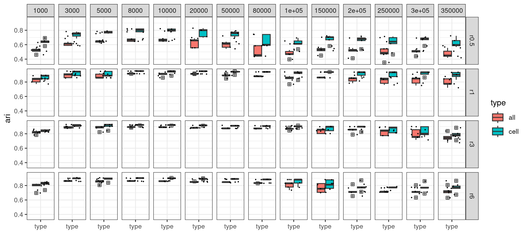
From the above ARI plot, we first observe when using radius 0.5, there is likely not enough neighborhood information and thus yield the worst performance.
Secondly, when we increase the number edges for training from 1,000 to 350,000, the stability of the ARI scores appears to increase at first but then drop when more edges were used, which is counter-intuitive.
We explore more
How many epochs have been applied
We can check how many epochs were actually applied for each training result.
## how many epochs eventually:

#output/test_radius/logs/nedges1000_repeats1_node_embs_r0.5.slurm.out
all_res_slurm_log <- list.files("output/test_radius/logs",
           pattern = "^nedges.*slurm.out",recursive = T,full.names = TRUE)
all_res_slurm_log <- all_res_slurm_log[!grepl("increase",all_res_slurm_log)]
#length(all_res_slurm_log)

# all_res_slurm_log <- all_res_slurm_log[!grepl("r0.5",
#                                               all_res_slurm_log)]

all_epoch_log <- lapply(all_res_slurm_log,
       function(file_name){
         #message(file_name)
         nedges = strsplit(basename(file_name),"_")[[1]][1]
         radius = strsplit(basename(file_name),"_")[[1]][5]
         rep = strsplit(basename(file_name),"_")[[1]][2]

         final_epochs = nrow(read.delim(file_name,header = FALSE)) -1
         data.frame(nedges,radius,rep,final_epochs)
         })
all_epoch_log <- do.call(rbind,all_epoch_log)
#all_epoch_log

all_epoch_log$nedges <- as.numeric(gsub("nedges","",all_epoch_log$nedges))
all_epoch_log$radius <- gsub(".slurm.out","",all_epoch_log$radius)
#acc_results_edge_effect_df
log_merged <- merge(acc_results_edge_effect_df,all_epoch_log)
p_high <- log_merged %>% group_by(type,radius,nedges,rep) %>%
arrange(-ari) %>%
slice(1) %>% ggplot()+
geom_boxplot(mapping = aes(x = type, y = ari,fill=type),
outlier.shape = 10)+
geom_jitter(mapping = aes(x = type, y = ari,color=final_epochs),
height = 0,
size = 2,
shape = 16)+
facet_grid(cols=vars(nedges),
rows=vars(radius))+
scale_colour_gradient2(low = "blue",
midpoint = 25,
high = "red")+
theme_bw(base_size = 12)+
theme(axis.title.x = element_blank())
p_high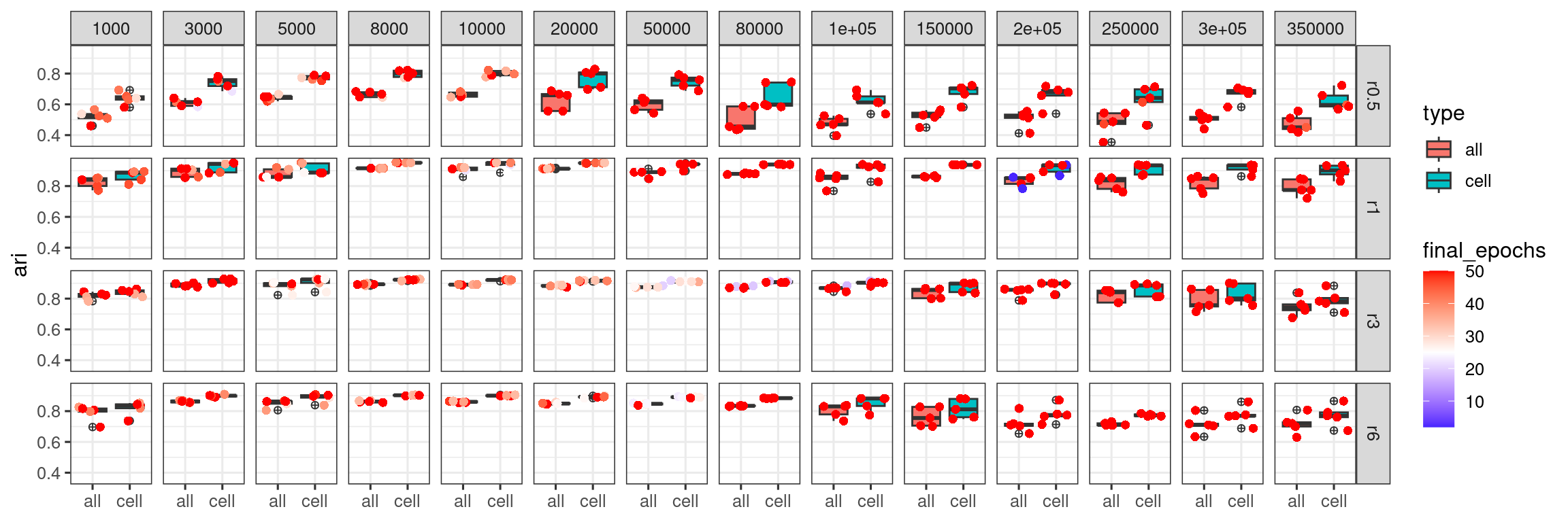
For the training outcomes obtained from using larger number of training edges, they seem more likely to reach the largest epoch 50. We next explore if we can bring up the stability of training for these cases by increasing total epochs.
Increase epochs
We next increase the maximum epoch number to 150, and we exclude radius 0.5 from the comparisons since they do not perform well overall due to the lack of spatial neighbors.
all_res_increasEpoch_for_more_edges <- list.files("output/test_radius",
                      pattern = "acc_r.*.csv",
                      recursive = TRUE,full.names = T)
all_res_increasEpoch_for_more_edges <-
  all_res_increasEpoch_for_more_edges[grepl("increase_epoch/",
                                            all_res_increasEpoch_for_more_edges)]
#length(all_res_increasEpoch_for_more_edges)

ari_res_increasEpoch_for_more_edges <-
  lapply(all_res_increasEpoch_for_more_edges,
       function(file_name){
         nedges = strsplit(file_name,"/")[[1]][3]
         radius = strsplit(file_name,"/")[[1]][6]
         rep = strsplit(file_name,"/")[[1]][5]
         acc_res = read.csv(file_name,header = 1,col.names = c("id","ari"))
         acc_res$nedges = nedges
         acc_res$rep <- rep

         acc_res$radius = radius
         acc_res[1:3,"id"] <- paste0("all_",acc_res[1:3,"id"])
         acc_res[4:6,"id"] <- paste0("cell_",acc_res[4:6,"id"])
         acc_res$type = c("all","all","all","cell","cell","cell")
         acc_res
       })

acc_results_inc_epochs_df <- do.call(rbind,ari_res_increasEpoch_for_more_edges)
acc_results_inc_epochs_df$nedges <- as.numeric(gsub("nedges","",
                                                     acc_results_inc_epochs_df$nedges))

acc_results_inc_epochs_df$radius <- gsub("acc_","",
                                          acc_results_inc_epochs_df$radius)
acc_results_inc_epochs_df$radius <- gsub(".csv","",
                                          acc_results_inc_epochs_df$radius)
## final epoch for increased epochs
all_res_slurm_log <- list.files("output/test_radius/logs",
pattern = "^nedges.*slurm.out",
recursive = T,full.names = TRUE)
all_res_slurm_log <- all_res_slurm_log[grepl("increase_epoch_repeats",
all_res_slurm_log)]
all_res_slurm_log <- all_res_slurm_log[!grepl("r0.5",all_res_slurm_log)]
#length(all_res_slurm_log)
all_epoch_log <- lapply(all_res_slurm_log,
function(file_name){
nedges = strsplit(basename(file_name),"_")[[1]][1]
radius = strsplit(basename(file_name),"_")[[1]][7]
rep = strsplit(basename(file_name),"_")[[1]][4]
final_epochs = nrow(read.delim(file_name,header = FALSE)) -1
data.frame(nedges,radius,rep,final_epochs)
})
all_epoch_log <- do.call(rbind,all_epoch_log)
all_epoch_log$nedges <- as.numeric(gsub("nedges","",all_epoch_log$nedges))
all_epoch_log$radius <- gsub(".slurm.out","",all_epoch_log$radius)
log_merged_inc_epochs <- merge(acc_results_inc_epochs_df,all_epoch_log)
p_high <- log_merged_inc_epochs %>%
group_by(type,radius,nedges,rep) %>%
arrange(-ari) %>%
slice(1) %>% ggplot()+
geom_boxplot(mapping = aes(x = type, y = ari,fill=type),
outlier.shape = 10)+
geom_jitter(mapping = aes(x = type, y = ari,color=final_epochs),
height = 0,
size = 2,
shape = 16)+
facet_grid(cols=vars(nedges),
rows=vars(radius))+
scale_colour_gradient2(low = "blue",
midpoint = 80,
high = "red")+
theme_bw(base_size = 12)+
theme(axis.title.x = element_blank())
p_high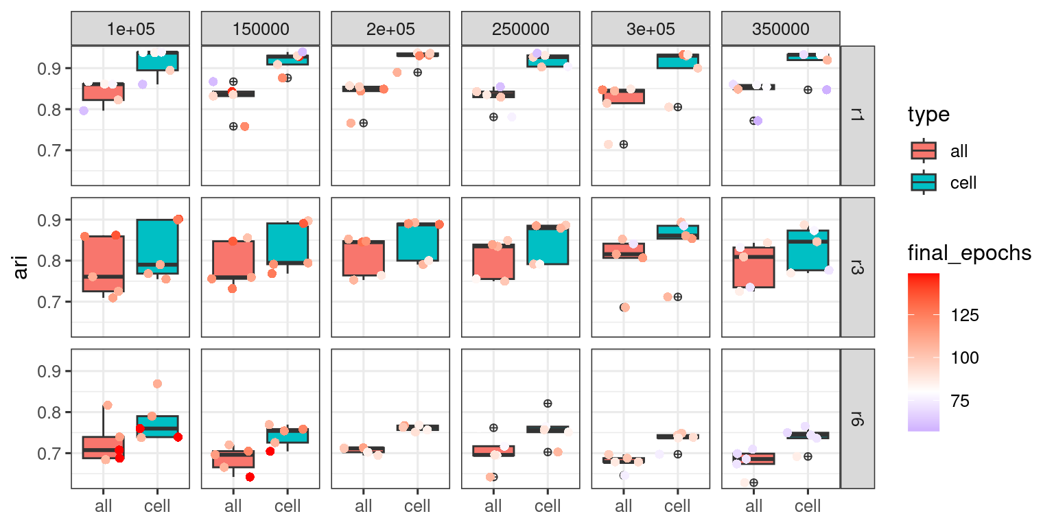
When we jointly view the max_epoch_50 and max_epoch_150 training results, we get the plot below.
log_merged_inc_epochs$train_type <- "max_150"
log_merged$train_type <- "max_50"

rbind(log_merged,log_merged_inc_epochs) %>%
  group_by(type,radius,nedges,rep,train_type) %>%
  arrange(-ari) %>%
  slice(1) %>%
  mutate(train_type = factor(train_type,
                             levels=c("max_50","max_150"))) %>% ggplot()+
  geom_boxplot(mapping = aes(x = type, y = ari,fill=type),
               outlier.shape = 10)+
  geom_jitter(mapping = aes(x = type, y = ari,color=final_epochs),
              height = 0,
              size = 2,
              shape = 16)+
  facet_grid(cols=vars(nedges,train_type),
             rows=vars(radius))+
  scale_colour_viridis_c()+
  theme_bw(base_size = 12)+
  theme(axis.title.x = element_blank())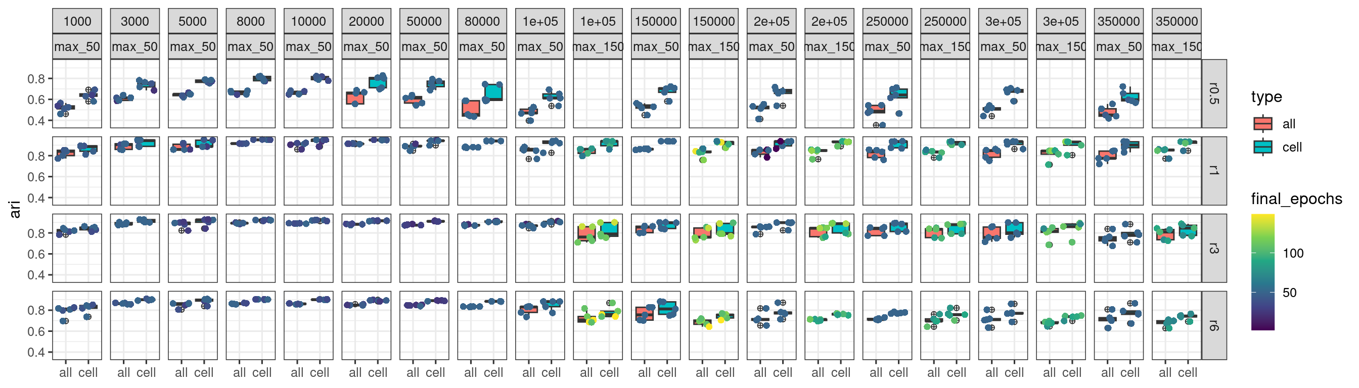
It appears more epoch runs have made training outcomes “worse” with reduced stability and ARI scores.
Increase batch size
For all the results presented above, we had applied training with a batch size of 100. We next explore how the batch size affects the training outcomes, and whether larger batch size helps with training stability.
all_res_increasB_for_more_edges <- list.files("output",
                      pattern = "acc_r.*.csv",
                      recursive = TRUE,full.names = T)
all_res_increasB_for_more_edges <- all_res_increasB_for_more_edges[grepl("increase_batch/",all_res_increasB_for_more_edges)]
#length(all_res_increasB_for_more_edges)

ari_res_increasB <- lapply(all_res_increasB_for_more_edges,
       function(file_name){
         nedges = strsplit(file_name,"/")[[1]][3]
         radius = strsplit(file_name,"/")[[1]][6]
         rep = strsplit(file_name,"/")[[1]][5]
         acc_res = read.csv(file_name,header = 1,col.names = c("id","ari"))
         acc_res$nedges = nedges
         acc_res$rep <- rep

         acc_res$radius = radius
         acc_res[1:3,"id"] <- paste0("all_",acc_res[1:3,"id"])
         acc_res[4:6,"id"] <- paste0("cell_",acc_res[4:6,"id"])
         acc_res$type = c("all","all","all","cell","cell","cell")
         acc_res
       })

acc_results_inc_batch400_df <- do.call(rbind,ari_res_increasB)
acc_results_inc_batch400_df$nedges <- as.numeric(gsub("nedges","",
                                                     acc_results_inc_batch400_df$nedges))

acc_results_inc_batch400_df$radius <- gsub("acc_","",
                                          acc_results_inc_batch400_df$radius)
acc_results_inc_batch400_df$radius <- gsub(".csv","",
                                          acc_results_inc_batch400_df$radius)
acc_results_inc_batch400_df %>%
group_by(type,radius,nedges,rep) %>%
arrange(-ari) %>%
slice(1) %>%
ggplot()+
geom_boxplot(mapping = aes(x = "type", y =ari,fill=type),
outlier.shape = 12)+
geom_jitter(mapping = aes(x = "type", y =ari),height = 0,
size=0.1)+
facet_grid(cols = vars(nedges),rows = vars(radius),
scales = "free_x",
space="free_x")+
theme_bw(base_size = 10)+
theme(axis.text.x = element_text(angle = 0),
axis.title.x = element_blank())+
ggtitle("max epoch 50, batch size 400")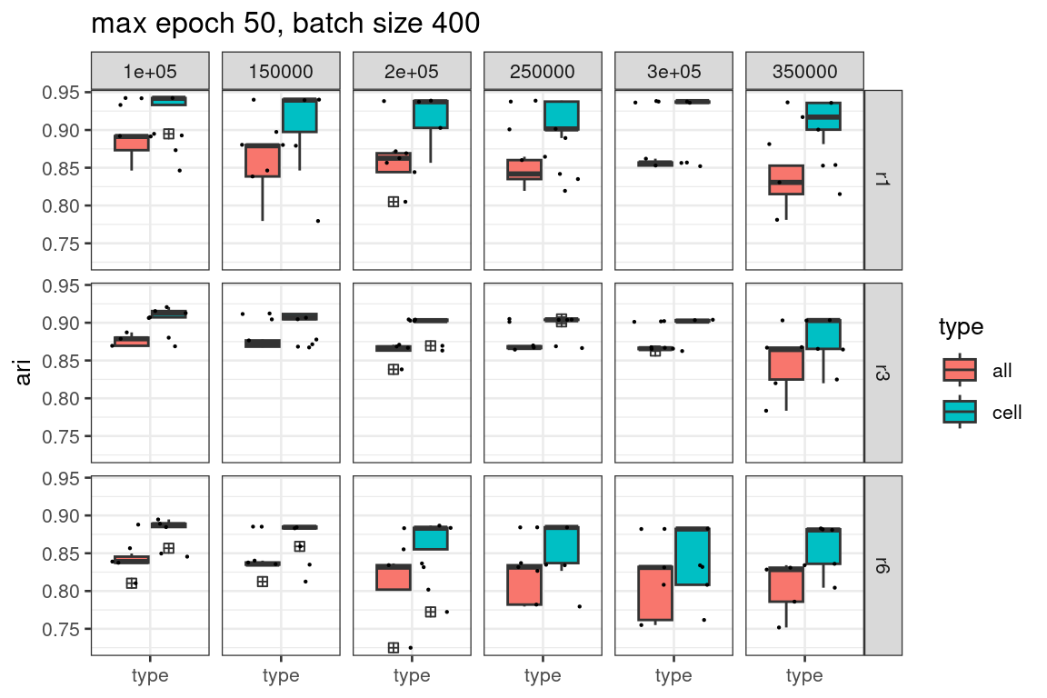
Increase batch size further to 800, 1200, as well as maximum epochs
all_res_increasB_for_more_edges <- list.files("output",
                      pattern = "acc_r.*.csv",
                      recursive = TRUE,
                      full.names = T)
all_res_increasB_for_more_edges <- all_res_increasB_for_more_edges[grepl("increase_epoch_batch",
                                                                         all_res_increasB_for_more_edges)]
#length(all_res_increasB_for_more_edges)

ari_res_increasB <- lapply(all_res_increasB_for_more_edges,
       function(file_name){
         nedges = strsplit(file_name,"/")[[1]][3]
         radius = strsplit(file_name,"/")[[1]][6]
         rep = strsplit(file_name,"/")[[1]][5]
         batch_size = strsplit(file_name,"/")[[1]][4]
         acc_res = read.csv(file_name,header = 1,col.names = c("id","ari"))
         acc_res$nedges = nedges
         acc_res$rep <- rep

         acc_res$radius = radius
         acc_res$batch_size = batch_size
         acc_res[1:3,"id"] <- paste0("all_",acc_res[1:3,"id"])
         acc_res[4:6,"id"] <- paste0("cell_",acc_res[4:6,"id"])
         acc_res$type = c("all","all","all","cell","cell","cell")
         acc_res
       })

acc_results_inc_b_df <- do.call(rbind,ari_res_increasB)
acc_results_inc_b_df$nedges <- as.numeric(gsub("nedges","",
                                                     acc_results_inc_b_df$nedges))

acc_results_inc_b_df$radius <- gsub("acc_","",
                                          acc_results_inc_b_df$radius)
acc_results_inc_b_df$radius <- gsub(".csv","",
                                          acc_results_inc_b_df$radius)

acc_results_inc_b_df$batch_size <- gsub("increase_epoch_","",
                                        acc_results_inc_b_df$batch_size )

acc_results_inc_b_df$batch_size <- factor(acc_results_inc_b_df$batch_size,
                                          levels=c("batch800","batch1200"))
acc_results_inc_b_df %>%
group_by(type,radius,nedges,rep,batch_size) %>%
arrange(-ari) %>%
slice(1) %>%
ggplot()+
geom_boxplot(mapping = aes(x = batch_size, y =ari,fill=type),
outlier.shape = 12)+
geom_jitter(mapping = aes(x = batch_size, y =ari),height = 0,
size=0.1)+
facet_grid(cols = vars(nedges),rows = vars(radius),
scales = "free_x",
space="free_x")+
theme_bw(base_size = 10)+
theme(axis.text.x = element_text(angle = 90),
axis.title.x = element_blank())+
ggtitle("max epoch 200, batch size 800,1200")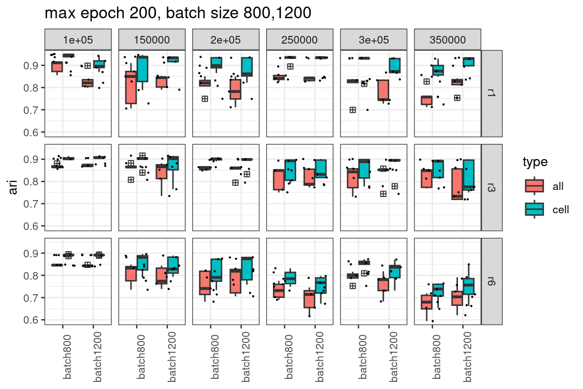
It is not convincing large batch size with more epochs of training is better from our evaluation.
Could it be due to overfitting?
We next train the models with 10 epochs only, and check the performance.
all_10epochs <- list.files("output/ten_epoch",
                      pattern = "ari_r.*.csv",
                      recursive = TRUE,
                      full.names = T)

#length(all_10epochs)

ari_res_10epochs_df <- lapply(all_10epochs,
       function(file_name){
         nedges = strsplit(file_name,"/")[[1]][3]
         radius = strsplit(file_name,"/")[[1]][5]
         rep = strsplit(file_name,"/")[[1]][4]
         acc_res = read.csv(file_name,header = 1,col.names = c("id","ari"))
         acc_res$nedges = nedges
         acc_res$rep <- rep

         acc_res$radius = radius
         acc_res[1:3,"id"] <- paste0("all_",acc_res[1:3,"id"])
         acc_res[4:6,"id"] <- paste0("cell_",acc_res[4:6,"id"])
         acc_res$type = c("all","all","all","cell","cell","cell")
         acc_res
       })

ari_res_10epochs_df <- do.call(rbind,ari_res_10epochs_df)
ari_res_10epochs_df %>%
group_by(type,radius,nedges,rep) %>%
arrange(-ari) %>%
slice(1) %>%
ggplot()+
geom_boxplot(mapping = aes(x = "type", y =ari,fill=type),
outlier.shape = 12)+
geom_jitter(mapping = aes(x = "type", y =ari),height = 0,
size=0.1)+
facet_grid(cols = vars(nedges),rows = vars(radius),
scales = "free_x",
space="free_x")+
theme_bw(base_size = 10)+
theme(axis.text.x = element_text(angle = 90),
axis.title.x = element_blank())+
ggtitle("10 epochs, batch size 100")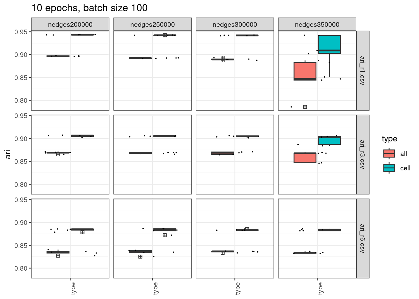
We see from the plot above, the stability has improved for 200k, 250k, and 300k edges but still not ideal for 350k when radius = 1, or 3.
A joint effect of fewer epochs and large batch size for stably trained models
After multiple rounds of investigation, we found increasing the batch size, and keep the number of training epochs to ~10 when using larger numbers of edges for training, the training results are stable with increasing number of edges used for training.
all_stable_gpu <- list.files("output/stable_train_gpu",
                      pattern = "ari_r.*.csv",
                      recursive = TRUE,
                      full.names = T)

#length(all_stable_gpu)

all_stable_gpu_df <- lapply(all_stable_gpu,
       function(file_name){
         nedges = strsplit(file_name,"/")[[1]][3]
         radius = strsplit(file_name,"/")[[1]][6]
         rep = strsplit(file_name,"/")[[1]][5]
         batch_size = strsplit(file_name,"/")[[1]][4]
         acc_res = read.csv(file_name,header = 1,
                            col.names = c("id","ari"))
         acc_res$nedges = nedges
         acc_res$rep <- rep

         acc_res$radius = radius
         acc_res$batch_size = batch_size

         acc_res[1:3,"id"] <- paste0("all_",acc_res[1:3,"id"])
         acc_res[4:6,"id"] <- paste0("cell_",acc_res[4:6,"id"])
         acc_res$type = c("all","all","all","cell","cell","cell")
         acc_res
       })

all_stable_gpu_df <- do.call(rbind,all_stable_gpu_df)
all_stable_gpu_df$radius <- gsub(".csv","",all_stable_gpu_df$radius)
all_stable_gpu_df$radius <- gsub("ari_","",all_stable_gpu_df$radius)
all_stable_gpu_df$nedges <- gsub("nedges","",all_stable_gpu_df$nedges)
all_stable_gpu_df$nedges <- factor(all_stable_gpu_df$nedges,
                                   levels = c("1000",
                                              "3000",
                                              "5000",
                                              "8000",
                                              "10000",
                                              "15000",
                                              "20000",
                                              "50000",
                                              "80000",
                                              "100000",
                                              "150000",
                                              "250000",
                                              "350000"))
all_stable_gpu_df %>%
group_by(type,radius,nedges,rep,batch_size) %>%
filter(radius !="r0.5")%>%
arrange(-ari) %>%
slice(1) %>%
ggplot()+
geom_boxplot(mapping = aes(x = radius, y =ari,fill=type),
outlier.shape = 12)+
geom_jitter(mapping = aes(x = radius, y =ari),height = 0,
size=0.1)+
facet_grid(cols = vars(nedges),
scales = "free_x",
space="free_x")+
theme_bw(base_size = 10)+
theme(axis.text.x = element_text(angle = 90),
axis.title.x = element_blank())+
ggtitle("10 epochs, batch size 1024")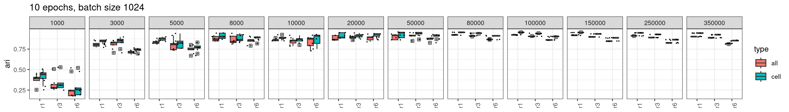
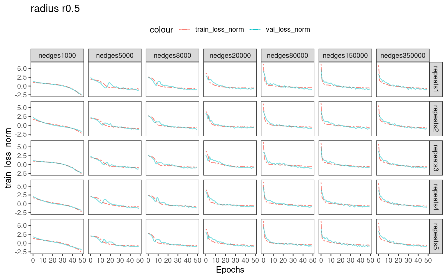
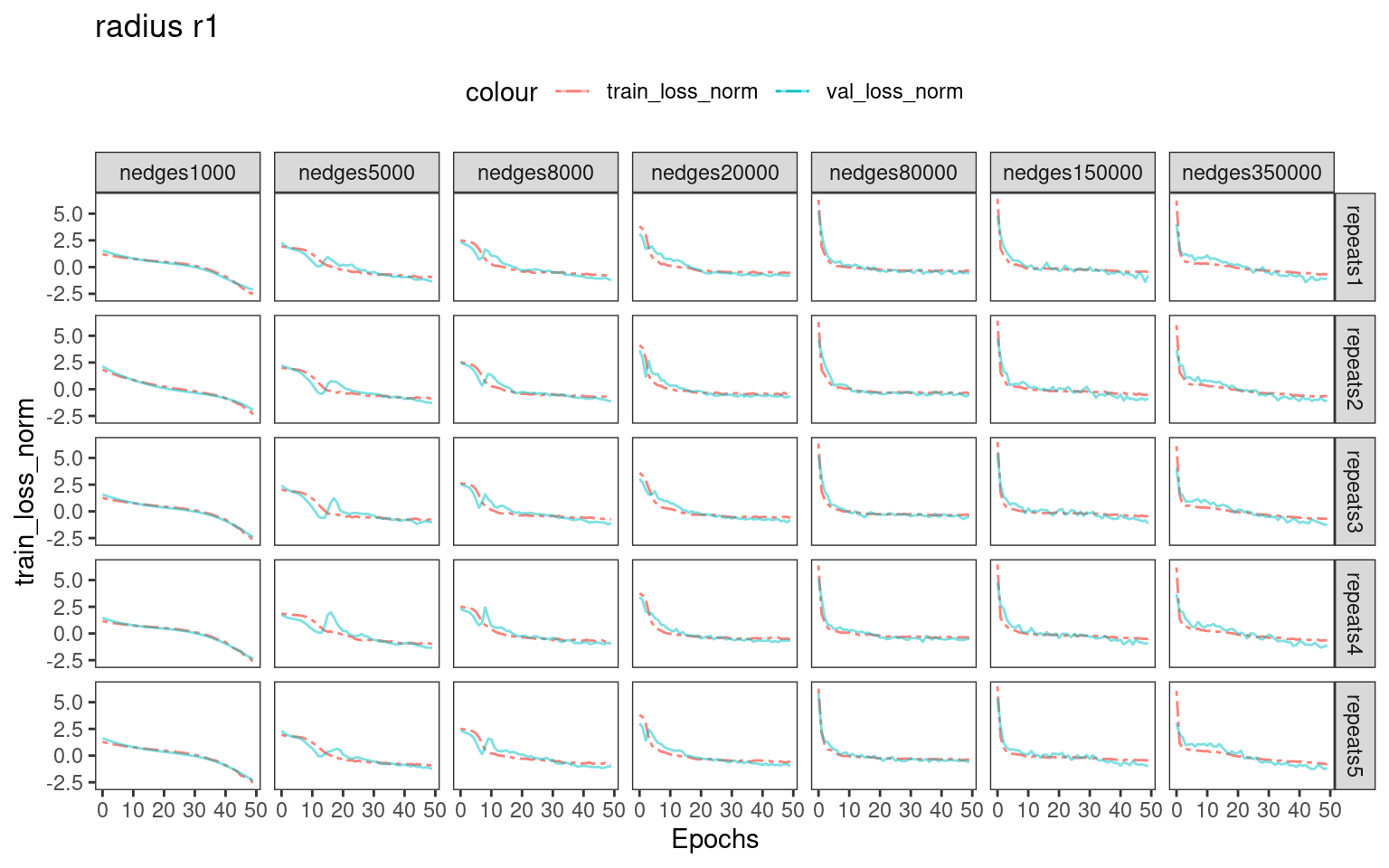
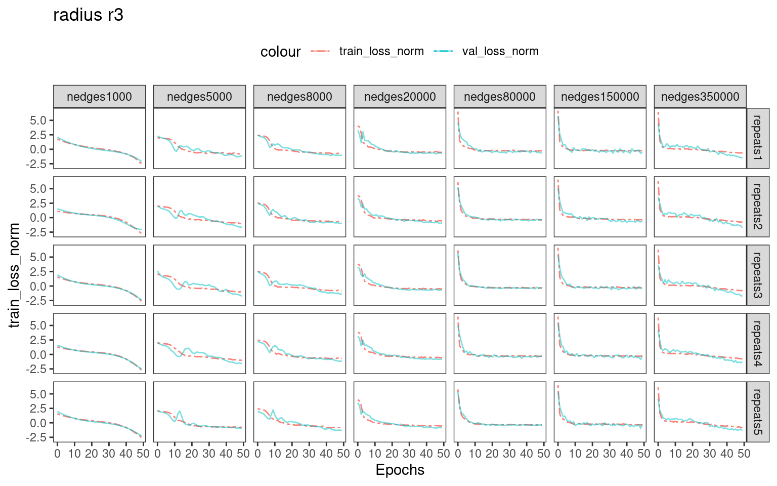
Choosing number of epochs based on training_loss and validation_loss curves
For real-world dataset analysis, there is no ground-truth labels for us to select an optional batch size and number epochs for training. We recommend inspecting the training and validation loss.
# batch 1024
# dim 50, 2 layers
# train 10 epochs for all

all_loss <- list.files("output/test_loss",
                      pattern = ".*.csv",
                      recursive = TRUE,full.names = T)

length(all_loss)
[1] 105loss_results <- lapply(all_loss,
function(file_name){
nedges = strsplit(file_name,"/")[[1]][3]
radius = strsplit(file_name,"/")[[1]][6]
rep = strsplit(file_name,"/")[[1]][5]
batchsize = strsplit(file_name,"/")[[1]][4]
arires = read.csv(file_name,header = 1)
arires$nedges = nedges
arires$rep <- rep
arires$batchsize <- batchsize
arires$radius = radius
arires
})
loss_result_df <- do.call(rbind, loss_results)
## rename. test_loss is actually val_loss
loss_result_df$val_loss <- loss_result_df$test_loss_list
loss_result_df$radius <- gsub("train_test_loss_","",loss_result_df$radius)
loss_result_df$radius <- gsub(".csv","",loss_result_df$radius)p_list = lapply(unique(loss_result_df$radius),
function(r){
loss_result_df %>% filter(radius == r) %>%
mutate(nedges = factor(nedges,
levels = c("nedges1000" ,"nedges5000" , "nedges8000",
"nedges20000","nedges80000", "nedges150000",
"nedges350000" ))) %>%
group_by(rep,nedges,radius) %>%
mutate(train_loss_norm = scale(train_loss),
val_loss_norm = scale(val_loss)) %>%
ggplot()+geom_line(mapping = aes(x = X, y = train_loss_norm,
color="train_loss_norm"),
linetype = "twodash",
linewidth = 0.5,
alpha = 0.9)+
geom_line(mapping = aes(x = X, y = val_loss_norm,
color = "val_loss_norm"),
linewidth = 0.5,alpha = 0.5)+
facet_grid(rows=vars(rep),
cols=vars(nedges))+
theme_bw()+
theme(legend.position = "top",
panel.grid = element_blank())+
xlab("Epochs")+
ggtitle(paste0("radius ", r))
})
# pdf("./output/figure_loss.pdf",onefile = TRUE, width = 14)
# print(gridExtra::marrangeGrob(p_list, nrow = 1, ncol = 1))
# dev.off()
We can see that when using larger number of edges for training, the training loss and validation loss drops rapidly in the first 5-10 epochs. Therefore, training with more epochs ( >>10 ) possibly introduces overfitting.
R version 4.1.2 (2021-11-01)
Platform: x86_64-pc-linux-gnu (64-bit)
Running under: Rocky Linux 8.10 (Green Obsidian)

Matrix products: default
BLAS/LAPACK: /usr/lib64/libopenblasp-r0.3.15.so

locale:
 [1] LC_CTYPE=en_AU.UTF-8       LC_NUMERIC=C
 [3] LC_TIME=en_AU.UTF-8        LC_COLLATE=en_AU.UTF-8
 [5] LC_MONETARY=en_AU.UTF-8    LC_MESSAGES=en_AU.UTF-8
 [7] LC_PAPER=en_AU.UTF-8       LC_NAME=C
 [9] LC_ADDRESS=C               LC_TELEPHONE=C
[11] LC_MEASUREMENT=en_AU.UTF-8 LC_IDENTIFICATION=C

attached base packages:
[1] stats     graphics  grDevices utils     datasets  methods   base

other attached packages:
[1] dplyr_1.1.3   plotly_4.10.4 ggplot2_3.4.4 readr_2.1.3

loaded via a namespace (and not attached):
 [1] tidyselect_1.2.0  xfun_0.41         bslib_0.5.1       purrr_1.0.2
 [5] colorspace_2.1-0  vctrs_0.6.4       generics_0.1.3    viridisLite_0.4.2
 [9] htmltools_0.5.7   yaml_2.3.7        utf8_1.2.4        rlang_1.1.2
[13] jquerylib_0.1.4   later_1.3.1       pillar_1.9.0      glue_1.6.2
[17] withr_2.5.2       lifecycle_1.0.3   stringr_1.5.0     munsell_0.5.0
[21] gtable_0.3.4      workflowr_1.7.0   htmlwidgets_1.6.2 evaluate_0.23
[25] labeling_0.4.3    knitr_1.45        tzdb_0.4.0        fastmap_1.1.1
[29] httpuv_1.6.12     fansi_1.0.5       highr_0.10        Rcpp_1.0.11
[33] promises_1.2.1    scales_1.3.0      cachem_1.0.8      jsonlite_1.8.7
[37] farver_2.1.1      fs_1.6.3          hms_1.1.2         digest_0.6.33
[41] stringi_1.7.12    rprojroot_2.0.3   grid_4.1.2        cli_3.6.1
[45] tools_4.1.2       magrittr_2.0.3    sass_0.4.7        lazyeval_0.2.2
[49] tibble_3.2.1      tidyr_1.3.0       pkgconfig_2.0.3   ellipsis_0.3.2
[53] data.table_1.14.8 rmarkdown_2.25    httr_1.4.7        rstudioapi_0.13
[57] R6_2.5.1          git2r_0.29.0      compiler_4.1.2
Warning in system("timedatectl", intern = TRUE): running command 'timedatectl'
had status 1
─ Session info ───────────────────────────────────────────────────────────────
setting value
version R version 4.1.2 (2021-11-01)
os Rocky Linux 8.10 (Green Obsidian)
system x86_64, linux-gnu
ui X11
language (EN)
collate en_AU.UTF-8
ctype en_AU.UTF-8
tz Australia/Melbourne
date 2024-08-20
pandoc 3.1.1 @ /usr/lib/rstudio-server/bin/quarto/bin/tools/ (via rmarkdown)
─ Packages ───────────────────────────────────────────────────────────────────
package * version date (UTC) lib source
brio 1.1.3 2021-11-30 [1] CRAN (R 4.1.2)
bslib 0.5.1 2023-08-11 [1] CRAN (R 4.1.2)
cachem 1.0.8 2023-05-01 [1] CRAN (R 4.1.2)
callr 3.7.0 2021-04-20 [1] CRAN (R 4.1.2)
cli 3.6.1 2023-03-23 [1] CRAN (R 4.1.2)
colorspace 2.1-0 2023-01-23 [1] CRAN (R 4.1.2)
crayon 1.5.2 2022-09-29 [1] CRAN (R 4.1.2)
data.table 1.14.8 2023-02-17 [1] CRAN (R 4.1.2)
desc 1.4.1 2022-03-06 [1] CRAN (R 4.1.2)
devtools 2.4.3 2021-11-30 [1] CRAN (R 4.1.2)
digest 0.6.33 2023-07-07 [1] CRAN (R 4.1.2)
dplyr * 1.1.3 2023-09-03 [1] CRAN (R 4.1.2)
ellipsis 0.3.2 2021-04-29 [1] CRAN (R 4.1.2)
evaluate 0.23 2023-11-01 [1] CRAN (R 4.1.2)
fansi 1.0.5 2023-10-08 [1] CRAN (R 4.1.2)
farver 2.1.1 2022-07-06 [1] CRAN (R 4.1.2)
fastmap 1.1.1 2023-02-24 [1] CRAN (R 4.1.2)
fs 1.6.3 2023-07-20 [1] CRAN (R 4.1.2)
generics 0.1.3 2022-07-05 [1] CRAN (R 4.1.2)
ggplot2 * 3.4.4 2023-10-12 [1] CRAN (R 4.1.2)
git2r 0.29.0 2021-11-22 [1] CRAN (R 4.1.2)
glue 1.6.2 2022-02-24 [1] CRAN (R 4.1.2)
gtable 0.3.4 2023-08-21 [1] CRAN (R 4.1.2)
highr 0.10 2022-12-22 [1] CRAN (R 4.1.2)
hms 1.1.2 2022-08-19 [1] CRAN (R 4.1.2)
htmltools 0.5.7 2023-11-03 [1] CRAN (R 4.1.2)
htmlwidgets 1.6.2 2023-03-17 [1] CRAN (R 4.1.2)
httpuv 1.6.12 2023-10-23 [1] CRAN (R 4.1.2)
httr 1.4.7 2023-08-15 [1] CRAN (R 4.1.2)
jquerylib 0.1.4 2021-04-26 [1] CRAN (R 4.1.2)
jsonlite 1.8.7 2023-06-29 [1] CRAN (R 4.1.2)
knitr 1.45 2023-10-30 [1] CRAN (R 4.1.2)
labeling 0.4.3 2023-08-29 [1] CRAN (R 4.1.2)
later 1.3.1 2023-05-02 [1] CRAN (R 4.1.2)
lazyeval 0.2.2 2019-03-15 [1] CRAN (R 4.1.2)
lifecycle 1.0.3 2022-10-07 [1] CRAN (R 4.1.2)
magrittr 2.0.3 2022-03-30 [1] CRAN (R 4.1.2)
memoise 2.0.1 2021-11-26 [1] CRAN (R 4.1.2)
munsell 0.5.0 2018-06-12 [1] CRAN (R 4.1.2)
pillar 1.9.0 2023-03-22 [1] CRAN (R 4.1.2)
pkgbuild 1.3.1 2021-12-20 [1] CRAN (R 4.1.2)
pkgconfig 2.0.3 2019-09-22 [1] CRAN (R 4.1.2)
pkgload 1.2.4 2021-11-30 [1] CRAN (R 4.1.2)
plotly * 4.10.4 2024-01-13 [1] CRAN (R 4.1.2)
prettyunits 1.1.1 2020-01-24 [1] CRAN (R 4.1.2)
processx 3.5.2 2021-04-30 [1] CRAN (R 4.1.2)
promises 1.2.1 2023-08-10 [1] CRAN (R 4.1.2)
ps 1.6.0 2021-02-28 [1] CRAN (R 4.1.2)
purrr 1.0.2 2023-08-10 [1] CRAN (R 4.1.2)
R6 2.5.1 2021-08-19 [1] CRAN (R 4.1.2)
Rcpp 1.0.11 2023-07-06 [1] CRAN (R 4.1.2)
readr * 2.1.3 2022-10-01 [1] CRAN (R 4.1.2)
remotes 2.4.2 2021-11-30 [1] CRAN (R 4.1.2)
rlang 1.1.2 2023-11-04 [1] CRAN (R 4.1.2)
rmarkdown 2.25 2023-09-18 [1] CRAN (R 4.1.2)
rprojroot 2.0.3 2022-04-02 [1] CRAN (R 4.1.2)
rstudioapi 0.13 2020-11-12 [1] CRAN (R 4.1.2)
sass 0.4.7 2023-07-15 [1] CRAN (R 4.1.2)
scales 1.3.0 2023-11-28 [1] CRAN (R 4.1.2)
sessioninfo 1.2.2 2021-12-06 [1] CRAN (R 4.1.2)
stringi 1.7.12 2023-01-11 [1] CRAN (R 4.1.2)
stringr 1.5.0 2022-12-02 [1] CRAN (R 4.3.0)
testthat 3.1.2 2022-01-20 [1] CRAN (R 4.1.2)
tibble 3.2.1 2023-03-20 [1] CRAN (R 4.1.2)
tidyr 1.3.0 2023-01-24 [1] CRAN (R 4.3.0)
tidyselect 1.2.0 2022-10-10 [1] CRAN (R 4.1.2)
tzdb 0.4.0 2023-05-12 [1] CRAN (R 4.1.2)
usethis 2.1.6 2022-05-25 [1] CRAN (R 4.1.2)
utf8 1.2.4 2023-10-22 [1] CRAN (R 4.1.2)
vctrs 0.6.4 2023-10-12 [1] CRAN (R 4.1.2)
viridisLite 0.4.2 2023-05-02 [1] CRAN (R 4.1.2)
withr 2.5.2 2023-10-30 [1] CRAN (R 4.1.2)
workflowr 1.7.0 2021-12-21 [1] CRAN (R 4.1.2)
xfun 0.41 2023-11-01 [1] CRAN (R 4.1.2)
yaml 2.3.7 2023-01-23 [1] CRAN (R 4.1.2)
[1] /mnt/beegfs/mccarthy/backed_up/general/rlyu/Software/Rlibs/4.1.2
[2] /opt/R/4.1.2/lib/R/library
──────────────────────────────────────────────────────────────────────────────