Pilot 3: Cell calling with lenti barcodes - donor 197
Christina Azodi
2022-05-03
Last updated: 2022-05-03
Checks: 5 2
Knit directory:
BAUH_2020_MND-single-cell/analysis/
This reproducible R Markdown analysis was created with workflowr (version 1.6.2). The Checks tab describes the reproducibility checks that were applied when the results were created. The Past versions tab lists the development history.
The R Markdown is untracked by Git. To know which version of the R
Markdown file created these results, you’ll want to first commit it to
the Git repo. If you’re still working on the analysis, you can ignore
this warning. When you’re finished, you can run
wflow_publish to commit the R Markdown file and build the
HTML.
Great job! The global environment was empty. Objects defined in the global environment can affect the analysis in your R Markdown file in unknown ways. For reproduciblity it’s best to always run the code in an empty environment.
The command set.seed(12345) was run prior to running the
code in the R Markdown file. Setting a seed ensures that any results
that rely on randomness, e.g. subsampling or permutations, are
reproducible.
Great job! Recording the operating system, R version, and package versions is critical for reproducibility.
Nice! There were no cached chunks for this analysis, so you can be confident that you successfully produced the results during this run.
Using absolute paths to the files within your workflowr project makes it difficult for you and others to run your code on a different machine. Change the absolute path(s) below to the suggested relative path(s) to make your code more reproducible.
| absolute | relative |
|---|---|
| /mnt/beegfs/mccarthy/backed_up/general/cazodi/Projects/BAUH_2020_MND-single-cell/output/pilot3_Lenti/03_keys/ | ../output/pilot3_Lenti/03_keys |
| /mnt/beegfs/mccarthy/backed_up/general/cazodi/Projects/BAUH_2020_MND-single-cell/output/pilot3.0_iPSC/ | ../output/pilot3.0_iPSC |
| /mnt/beegfs/mccarthy/backed_up/general/cazodi/Projects/BAUH_2020_MND-single-cell/output/pilot3.0_MN/ | ../output/pilot3.0_MN |
Great! You are using Git for version control. Tracking code development and connecting the code version to the results is critical for reproducibility.
The results in this page were generated with repository version 8ac0d8a. See the Past versions tab to see a history of the changes made to the R Markdown and HTML files.
Note that you need to be careful to ensure that all relevant files for
the analysis have been committed to Git prior to generating the results
(you can use wflow_publish or
wflow_git_commit). workflowr only checks the R Markdown
file, but you know if there are other scripts or data files that it
depends on. Below is the status of the Git repository when the results
were generated:
Ignored files:
    Ignored:    .RData
    Ignored:    .Rhistory
    Ignored:    .Rproj.user/
    Ignored:    .cache/
    Ignored:    .config/
    Ignored:    .snakemake/
    Ignored:    20220422_tSNE_plots.pdf
    Ignored:    BAUH_2020_MND-single-cell.Rproj
    Ignored:    GRCh38_turboGFP-RFP_reference/
    Ignored:    Homo_sapiens.GRCh38.turboGFP/
    Ignored:    Rplots.pdf
    Ignored:    analysis/2022-04-22_pilot2_CelltypeAbundance.pdf
    Ignored:    data/1-s2.0-S0002929720300781-main.pdf
    Ignored:    data/2103.11251.pdf
    Ignored:    data/3M-february-2018.txt
    Ignored:    data/737K-august-2016.txt
    Ignored:    data/Cellecta-SEQ-CloneTracker-XP_14bp_barcodes.txt
    Ignored:    data/Cellecta-SEQ-CloneTracker-XP_30bp_barcodes.txt
    Ignored:    data/STAR_index/
    Ignored:    data/STAR_output/
    Ignored:    data/donor_metadata.txt
    Ignored:    data/genome1K.phase3.SNP_AF5e2.chr1toX.hg38.log
    Ignored:    data/genome1K.phase3.SNP_AF5e2.chr1toX.hg38.recode.sort.vcf.gz
    Ignored:    data/genome1K.phase3.SNP_AF5e2.chr1toX.hg38.recode.sort.vcf.gz.csi
    Ignored:    data/genome1K.phase3.SNP_AF5e2.chr1toX.hg38.recode.vcf.gz
    Ignored:    data/genome1K.phase3.SNP_AF5e2.chr1toX.hg38.sort.vcf.gz
    Ignored:    data/genome1K.phase3.SNP_AF5e2.chr1toX.hg38.sort.vcf.gz.csi
    Ignored:    data/genome1K.phase3.SNP_AF5e2.chr1toX.hg38.vcf.gz
    Ignored:    data/genome1k.chr22.log
    Ignored:    data/genome1k.chr22.recode.vcf
    Ignored:    data/pilot2_donors.txt
    Ignored:    data/pilot3_aggr-experiments.csv
    Ignored:    data/pilot3_donors.txt
    Ignored:    data/pilot3_lenti_barcodes_capture5_poolA_D42pass.txt
    Ignored:    data/s41588-018-0268-8.pdf
    Ignored:    data/tr2g_hs.tsv
    Ignored:    logs/
    Ignored:    output/2021-04-27_pilot2_nCells-per-donor.pdf
    Ignored:    output/2021-08-03_pilot2_nCells-per-donor.pdf
    Ignored:    output/CB-scRNAv31-GEX-lib01_QC_metadata.txt
    Ignored:    output/CB-scRNAv31-GEX-lib02_QC_metadata.txt
    Ignored:    output/pilot1_starsoloED/
    Ignored:    output/pilot2.1_gex/
    Ignored:    output/pilot2_HTO-2/
    Ignored:    output/pilot2_HTO/
    Ignored:    output/pilot2_gex_MAF01-152/
    Ignored:    output/pilot2_gex_MAF01/
    Ignored:    output/pilot2_gex_starsolo/
    Ignored:    output/pilot2_gex_starsoloED_GFP/
    Ignored:    output/pilot3.0_MN/
    Ignored:    output/pilot3.0_iPSC/
    Ignored:    output/pilot3.1_iPSC/
    Ignored:    output/pilot3_Lenti/
    Ignored:    references/Homo_sapiens.GRCh38.turboGFP.bed
    Ignored:    references/Homo_sapiens.GRCh38.turboGFP.fa
    Ignored:    references/Homo_sapiens.GRCh38.turboGFP.fa.fai
    Ignored:    references/Homo_sapiens.GRCh38.turboGFP.filtered.gtf
    Ignored:    references/Homo_sapiens.GRCh38.turboGFP.gtf
    Ignored:    references/Homo_sapiens.GRCh38.turboGFP_gene.gtf
    Ignored:    references/SAindex/
    Ignored:    references/allen_brain_reference/
    Ignored:    references/geno_test.vcf.gz
    Ignored:    references/pilot3/
    Ignored:    references/pilot3_20220330/
    Ignored:    references/test
    Ignored:    references/turboGFP.fa
    Ignored:    references/turboGFP.gtf
    Ignored:    references/turboRFP.fa
    Ignored:    workflow/rules/

Untracked files:
    Untracked:  .nv/
    Untracked:  analysis/2022-04-08_pilot2_hg38-fix.Rmd
    Untracked:  analysis/2022-04-18_pilot3_capture3_SoupX.Rmd
    Untracked:  analysis/2022-04-18_pilot3_ipsc_SoupX.Rmd
    Untracked:  analysis/2022-04-22_pilot2_CelltypeAbundance.Rmd
    Untracked:  analysis/2022-05-03_pilot3_Cell-demultiplexing-Lenti.Rmd
    Untracked:  analysis/2022_04_08_pilot2_CellCalling-comparison.Rmd
    Untracked:  analysis/2022_04_15_pilot2_DE.Rmd
    Untracked:  cellbender.dockerfile
    Untracked:  code/.ipynb_checkpoints/
    Untracked:  code/run_soupX_pilot3_capture3.R
    Untracked:  code/souporcell_latest.sif
    Untracked:  code/subsetting_mpileup.R
    Untracked:  glimma-plots/
    Untracked:  hwe1e-05_maf05_vcf_stats.txt
    Untracked:  hwe1e-05_vcf_stats.txt
    Untracked:  workflow/Snakefile_simple.smk

Unstaged changes:
    Modified:   .gitignore
    Modified:   analysis/2021-09-29_pilot2_VireoResults.Rmd
    Modified:   analysis/2022-03-06_pilot3_CellQC.Rmd
    Modified:   analysis/index.Rmd
    Modified:   code/run_soupX_2.R
    Modified:   config/config_pilot3.0_MN.yml
    Modified:   config/config_pilot3.0_iPSC.yml
    Modified:   workflow/demuxlet_jobs/demux_capture5.sh
    Modified:   workflow/rules_prepare-genotype-data.smk
Note that any generated files, e.g. HTML, png, CSS, etc., are not included in this status report because it is ok for generated content to have uncommitted changes.
There are no past versions. Publish this analysis with
wflow_publish() to start tracking its development.
Overview of strategy
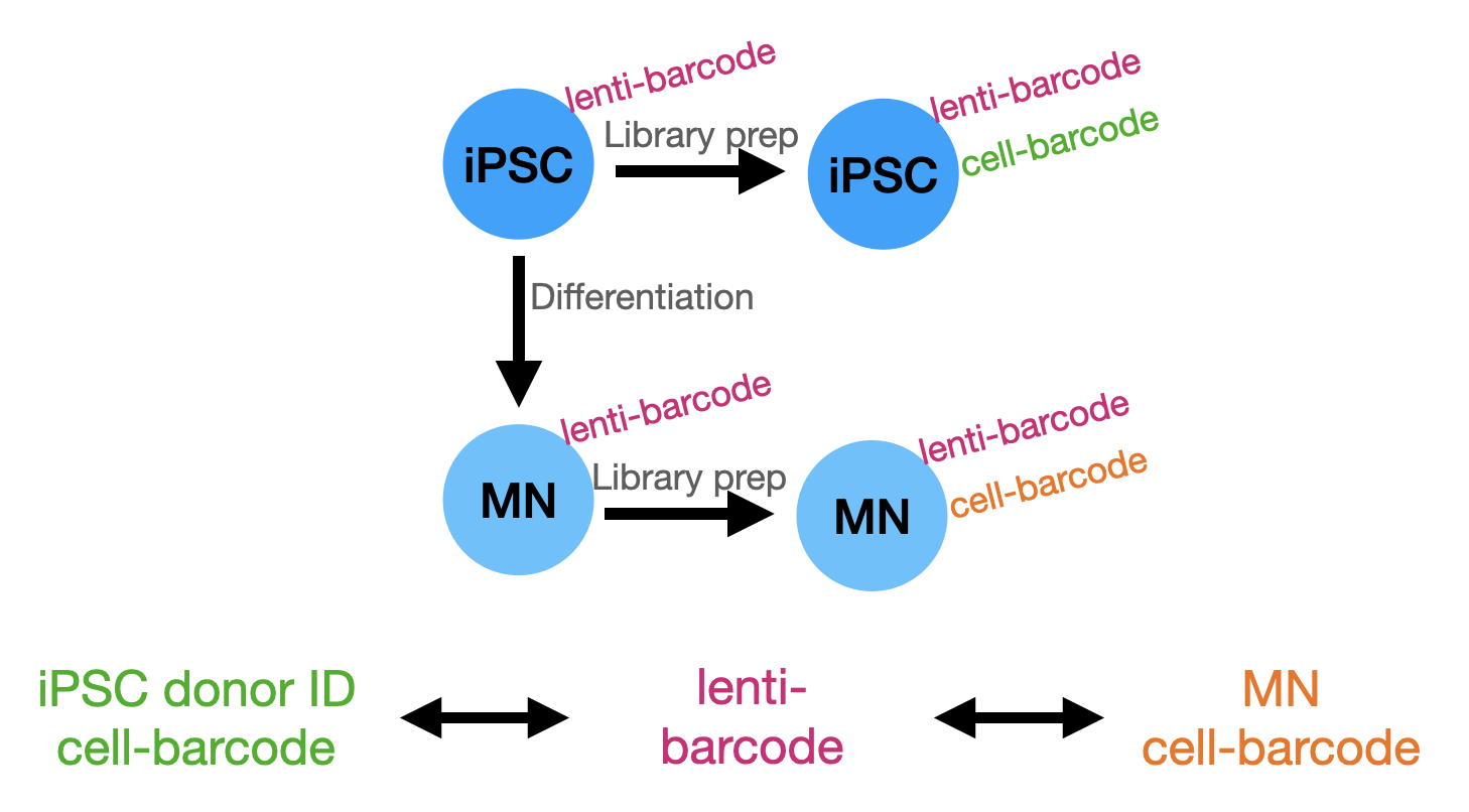
Using vireo and demuxlet for cell demultiplexing we find that donor 197 dominates the cell population, accounting for between 35-45% of cells. If the 150 donors co-cultured evenly, we’d expect ~ 0.7% of cells from each donor. This enrichment of donor 197 cells was observed using either tool, with various SNP filterings applied, when using vireo in the genotype guided or unguided settings, and futher if donor 197 was removed from the genotype reference provided, the majority of donor 197 cells became unassigned. This supports the hypothesis that the scRNA-seq data is dominated by reads from donor 197 cells. Because Chris also performed some DNA-seq experiments on the co-cultures to test the lenti barcode approach, we can see if the donor-197 associated lenti barcodes are enriched in the sample as well.
Comparing lenti-barcode map to called cells
First assessing how often called cells (by cellranger for now, but eventually using the ensemble cell calling approach) were also assigned lenti barcodes for Capture 4 and 5 separately. Action item: rerun this with the iPSC cells after increasing the cell threshold on cellbender - a quick test showed that if I included all barcodes called as cells by 2+ methods for the iPSCs, then about 90% of lenti barcoded cell barcodes were a called iPSC!
c5_lenti_key <- read.csv(paste0(lenti_dir, "Capture5-Lenti_cellbarcodes.tsv"),
                      sep = "\t")

c5_lenti_key <- c5_lenti_key %>% separate_rows(cell_barcodes, sep=";", convert = TRUE) %>%
  mutate(cell_barcodes = paste0(cell_barcodes, "-1"))

c5_cellbarcodes <- scan(paste0(ipsc_dir, "01_cellcalling-merged/Capture5-GEX/barcodes.txt"), what="character")

c5_ovlp <- table(c5_lenti_key$cell_barcodes %in% c5_cellbarcodes)

message("lenti barcodes that belong to a called iPSC: ", c5_ovlp[["TRUE"]], " (", round(c5_ovlp[["TRUE"]]/nrow(c5_lenti_key)*100, 1), "%)")
lenti barcodes that belong to a called iPSC: 309 (0.3%)However, this is still a relatively small proportion of called cells in both captures:
c5_ovlp2 <- table(c5_cellbarcodes %in% c5_lenti_key$cell_barcodes)

message("Called iPSCs with a lenti barcode: ", c5_ovlp2[["TRUE"]], " (", round(c5_ovlp2[["TRUE"]]/length(c5_cellbarcodes)*100, 1), "%)")
Called iPSCs with a lenti barcode: 309 (0.9%)Comparison with donor calls from vireo
Multiple cells may have the same lenti-barcode, but all of these cells should be from the same donor.
iPSCs (Capture 5)
First, merge the lenti-barcode information with the donor calls from vireo for the iPSCs. How many donors are assigned to each lenti-barcode?
ipsc_donors <- read.csv(paste0(ipsc_dir, "03_vireo-protCod-autos/donor_ids.tsv"), sep="\t")
ipsc_donors$cell_barcodes <- ipsc_donors$cell
sort(table(ipsc_donors$donor_id))
       101        117        120        141        145        199        232
         1          1          1          1          1          1          1
       723        745         77         84         89       W058       W093
         1          1          1          1          1          1          1
      W103        186        200        202        750        796         87
         1          2          2          2          2          2          2
      W001       W113       W221        138        142        146        191
         2          2          2          3          3          3          3
       239       T232        217         75         82         99        110
         3          3          4          4          4          4          5
       188         74         90       W104       W134        797   donor138
         5          5          5          5          5          6          6
  donor143       T233        121        130        208        113       W162
         6          6          7          7          7          8          8
      W263        240        118        231         93   donor140   donor148
         8          9         11         11         11         11         11
  donor149   donor141       W222        131   donor136   donor144        124
        11         12         12         13         13         13         14
  donor142   donor145   donor146   donor137        220       T234   donor147
        14         14         14         15         16         17         18
       196   donor139        105        238       W112         76        194
        19         19         20         20         20         22         24
       221        123        227       W014         92        102        214
        26         30         36         43         52         60         60
       237        107        127        192        104        210        190
        65         66         75        112        125        129        149
      W005        218        128       W187        189        187        122
       163        175        191        192        195        201        236
       207        100         88       W132        154        198        119
       236        246        348        438        650        693        775
       129    doublet        197 unassigned
      3304       5537       7653      11591
ipsc_donors <- ipsc_donors %>% left_join(c5_lenti_key[, c("lenti_bc", "cell_barcodes")],
by="cell_barcodes")
ipsc_donors_lenti <- na.omit(ipsc_donors)
message(length(unique(ipsc_donors_lenti$lenti_bc)), " lenti barcodes map to ",
length(unique(ipsc_donors_lenti$cell_barcodes)), " iPSCs") 118 lenti barcodes map to 309 iPSCsipsc_donors_lenti <- subset(ipsc_donors_lenti, ! donor_id %in% c("unassigned", "doublet") )
message(length(unique(ipsc_donors_lenti$lenti_bc)), " lenti barcodes map to ",
length(unique(ipsc_donors_lenti$cell_barcodes)), " iPSCs with donor IDs from vireo.") 80 lenti barcodes map to 197 iPSCs with donor IDs from vireo.summary_ipsc_donors_lenti <- ipsc_donors_lenti %>%
group_by(donor_id, lenti_bc) %>% tally() %>% group_by(lenti_bc) %>%
tally()
message("Number of lenti barcodes mapping to n donor IDs:")Number of lenti barcodes mapping to n donor IDs:table(summary_ipsc_donors_lenti$n)
 1  2  3 17
65 13  1  1
For lenti barcodes associated with more than one donor, what proportion (text=count) of cells are assigned to different donors?
inspect_bcs <- subset(summary_ipsc_donors_lenti, n > 1)$lenti_bc

ipsc_donors_lenti %>%
  dplyr::filter(lenti_bc %in% inspect_bcs) %>%
  ggplot(aes(fill=donor_id, x=lenti_bc)) +
  geom_bar(position="fill") +
  scale_y_continuous(labels = scales::percent, breaks = c(0, 0.2, 0.4, 0.6, 0.8, 1)) +
  theme_cowplot() +
  geom_text(stat="count", aes(label=ifelse((..count..)>0, ..count.., "")),
           position = position_fill(vjust=0.5)) +
  coord_flip()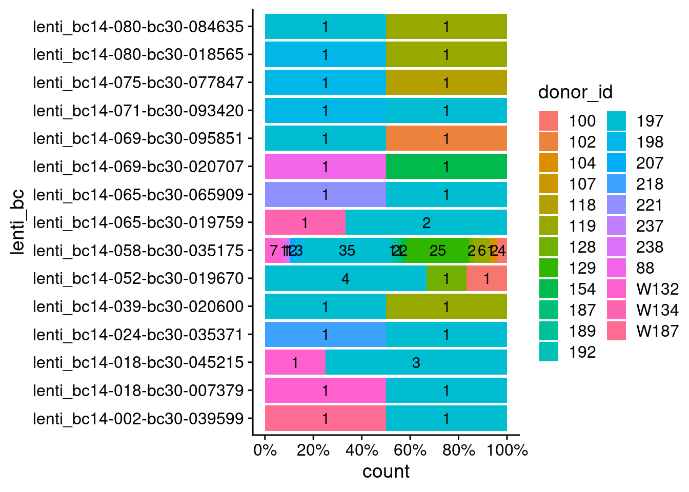
Number of cell barcodes (x-axis) associated with different donors (fill color) for each lenti barcode (y-axis).
Ignoring these lenti barcodes with ambiguous donor IDs, can we use the other lenti barcodes to assign donorIDs to more cells? Cells called as doublets by vireo should remain doublets, but for those that were unassigned by vireo, how many could we assign using a lenti barcode and how often do the lenti assignments match the best singlet estimated by vireo? This may give us a sense of how well we will be able to do this in MN cells…
good_lenti_barcodes <- subset(summary_ipsc_donors_lenti, n == 1)$lenti_bc
lenti_donor_key <- subset(ipsc_donors_lenti, lenti_bc %in% good_lenti_barcodes) %>%
  distinct(lenti_bc, donor_id)


ipsc_donors <- ipsc_donors %>% left_join(lenti_donor_key, by = "lenti_bc", suffix=c("", ".lenti"))
ipsc_donors_no_vireoID <- subset(ipsc_donors, donor_id %in% c("unassigned"))
x <- nrow(ipsc_donors_no_vireoID)
ipsc_donors_no_vireoID <- subset(ipsc_donors_no_vireoID, !is.na(donor_id.lenti))
x2 <- nrow(ipsc_donors_no_vireoID)
res <- table(ipsc_donors_no_vireoID$best_singlet == ipsc_donors_no_vireoID$donor_id.lenti)
message("Of ", x, " unassigned cells, ", x2, " have are associated with an unambiguous lenti barcodes and of those, ", res[["TRUE"]],  " (", round(res[["TRUE"]]/x2*100, 1),"%) are the same as the best singlet estimated by vireo.")
Of 11591 unassigned cells, 9 have are associated with an unambiguous lenti barcodes and of those, 2 (22.2%) are the same as the best singlet estimated by vireo.Inspecting donor 197
Does donor 197 have a proportionately large number of lenti barcodes? Or did a very large number of cells come from a single (lenti barcoded) progenitor?
ipsc_donors %>% group_by(donor_id) %>%
  dplyr::filter(!donor_id %in% c("doublet", "unassigned")) %>%
  summarise(n_cells = n(),
            n_lentiBCs = length(unique(lenti_bc))) %>%
  ggscatter(x="n_lentiBCs", y="n_cells", label = "donor_id", repel = TRUE, add = "reg.line")
`geom_smooth()` using formula 'y ~ x'Warning: ggrepel: 102 unlabeled data points (too many overlaps). Consider
increasing max.overlaps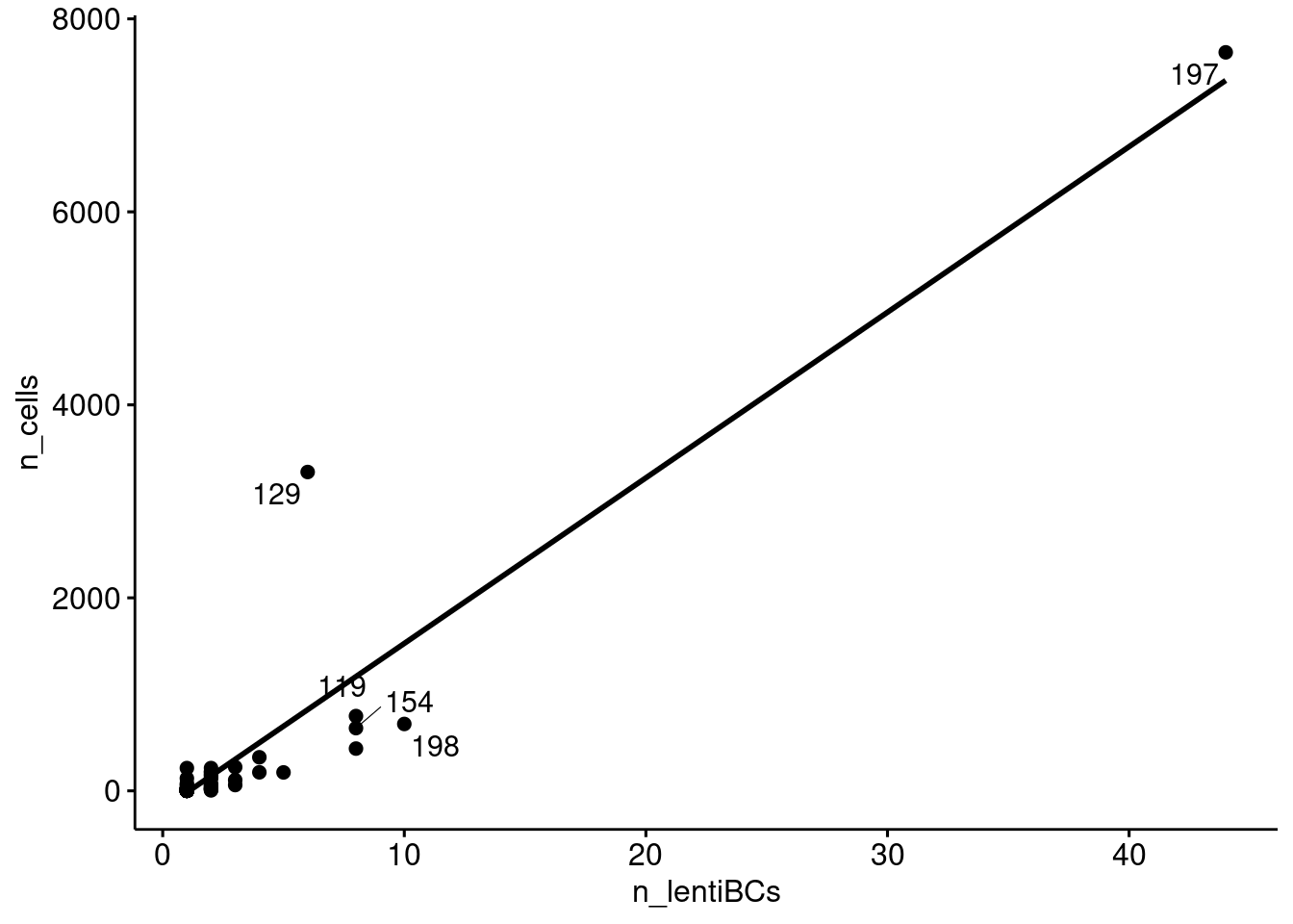
Relationship between the number of cells assigned to a donor and the number of lenti barcodes assigned to a donor.
d197 <- ipsc_donors %>% dplyr::filter(donor_id == "197")
d197_lbc_counts <- as.data.frame(table(d197$lenti_bc))
summary(d197_lbc_counts$Freq)
Min. 1st Qu. Median Mean 3rd Qu. Max.
1.000 1.000 1.000 1.953 1.000 35.000 message("Number of lenti-barcodes associated with donor 197: ", nrow(d197_lbc_counts))Number of lenti-barcodes associated with donor 197: 43write.table(d197_lbc_counts, paste0(lenti_dir, "20220503_donor197_lenti_barcodes.txt"),
row.names = FALSE, quote=FALSE)
sessionInfo()R version 4.1.1 (2021-08-10)
Platform: x86_64-pc-linux-gnu (64-bit)
Running under: Rocky Linux 8.5 (Green Obsidian)
Matrix products: default
BLAS/LAPACK: /usr/lib64/libopenblasp-r0.3.12.so
locale:
[1] LC_CTYPE=en_AU.UTF-8 LC_NUMERIC=C
[3] LC_TIME=en_AU.UTF-8 LC_COLLATE=en_AU.UTF-8
[5] LC_MONETARY=en_AU.UTF-8 LC_MESSAGES=en_AU.UTF-8
[7] LC_PAPER=en_AU.UTF-8 LC_NAME=C
[9] LC_ADDRESS=C LC_TELEPHONE=C
[11] LC_MEASUREMENT=en_AU.UTF-8 LC_IDENTIFICATION=C
attached base packages:
[1] stats graphics grDevices utils datasets methods base
other attached packages:
[1] viridis_0.6.2 viridisLite_0.4.0 cowplot_1.1.1 ggpubr_0.4.0
[5] ggplot2_3.3.5 data.table_1.14.2 tidyr_1.1.4 dplyr_1.0.7
[9] argparse_2.1.3
loaded via a namespace (and not attached):
[1] ggrepel_0.9.1 Rcpp_1.0.8 lattice_0.20-45 assertthat_0.2.1
[5] rprojroot_2.0.2 digest_0.6.29 utf8_1.2.2 R6_2.5.1
[9] backports_1.4.1 evaluate_0.15 highr_0.9 pillar_1.6.4
[13] rlang_1.0.2 rstudioapi_0.13 car_3.0-12 jquerylib_0.1.4
[17] Matrix_1.4-0 rmarkdown_2.11 labeling_0.4.2 splines_4.1.1
[21] stringr_1.4.0 munsell_0.5.0 broom_0.7.10 compiler_4.1.1
[25] httpuv_1.6.5 xfun_0.30 pkgconfig_2.0.3 mgcv_1.8-39
[29] htmltools_0.5.2 tidyselect_1.1.2 tibble_3.1.6 gridExtra_2.3
[33] workflowr_1.6.2 fansi_1.0.0 crayon_1.5.0 withr_2.5.0
[37] later_1.3.0 grid_4.1.1 nlme_3.1-152 jsonlite_1.8.0
[41] gtable_0.3.0 lifecycle_1.0.1 DBI_1.1.2 git2r_0.29.0
[45] magrittr_2.0.2 scales_1.1.1 cli_3.2.0 stringi_1.7.6
[49] carData_3.0-5 farver_2.1.0 ggsignif_0.6.3 fs_1.5.2
[53] promises_1.2.0.1 bslib_0.3.1 ellipsis_0.3.2 generics_0.1.2
[57] vctrs_0.3.8 tools_4.1.1 glue_1.6.0 purrr_0.3.4
[61] abind_1.4-5 fastmap_1.1.0 yaml_2.3.5 colorspace_2.0-3
[65] rstatix_0.7.0 knitr_1.37 sass_0.4.0