BIOS_analysis-workflow
Ruqian Lyu, Christina Azodi, Jeffrey Pullin
11/4/2020
Last updated: 2020-11-30
Checks: 6 1
Knit directory: bios_2020_single-cell-workshop-svi/
This reproducible R Markdown analysis was created with workflowr (version 1.6.2). The Checks tab describes the reproducibility checks that were applied when the results were created. The Past versions tab lists the development history.
The R Markdown file has unstaged changes. To know which version of the R Markdown file created these results, you’ll want to first commit it to the Git repo. If you’re still working on the analysis, you can ignore this warning. When you’re finished, you can run wflow_publish to commit the R Markdown file and build the HTML.
Great job! The global environment was empty. Objects defined in the global environment can affect the analysis in your R Markdown file in unknown ways. For reproduciblity it’s best to always run the code in an empty environment.
The command set.seed(20190102) was run prior to running the code in the R Markdown file. Setting a seed ensures that any results that rely on randomness, e.g. subsampling or permutations, are reproducible.
Great job! Recording the operating system, R version, and package versions is critical for reproducibility.
Nice! There were no cached chunks for this analysis, so you can be confident that you successfully produced the results during this run.
Great job! Using relative paths to the files within your workflowr project makes it easier to run your code on other machines.
Great! You are using Git for version control. Tracking code development and connecting the code version to the results is critical for reproducibility.
The results in this page were generated with repository version b0c7d78. See the Past versions tab to see a history of the changes made to the R Markdown and HTML files.
Note that you need to be careful to ensure that all relevant files for the analysis have been committed to Git prior to generating the results (you can use wflow_publish or wflow_git_commit). workflowr only checks the R Markdown file, but you know if there are other scripts or data files that it depends on. Below is the status of the Git repository when the results were generated:
Ignored files:
    Ignored:    .Rhistory
    Ignored:    .Rproj.user/

Untracked files:
    Untracked:  .Renviron
    Untracked:  Rcode.R
    Untracked:  Rcode2.R
    Untracked:  Rplots.pdf
    Untracked:  analysis/about.Rmd
    Untracked:  analysis/figure/
    Untracked:  analysis/license.Rmd
    Untracked:  data/
    Untracked:  memusage.txt
    Untracked:  raw_data/
    Untracked:  rscript.R
    Untracked:  untar_path/

Unstaged changes:
    Modified:   analysis/BIOS_analysis-workflow.Rmd
    Modified:   analysis/BIOS_dataset-source.Rmd
    Modified:   analysis/BIOS_sctransform-normalisation.Rmd
    Modified:   analysis/_site.yml
    Modified:   bios.bib
Note that any generated files, e.g. HTML, png, CSS, etc., are not included in this status report because it is ok for generated content to have uncommitted changes.
These are the previous versions of the repository in which changes were made to the R Markdown (analysis/BIOS_analysis-workflow.Rmd) and HTML (public/BIOS_analysis-workflow.html) files. If you’ve configured a remote Git repository (see ?wflow_git_remote), click on the hyperlinks in the table below to view the files as they were in that past version.
| File | Version | Author | Date | Message |
|---|---|---|---|---|
| Rmd | b0c7d78 | rlyu | 2020-11-27 | description of number of HVGs to keep |
| html | 1f42bf1 | rlyu | 2020-11-27 | J’s edits |
| Rmd | 0c058e2 | rlyu | 2020-11-27 | small edits |
| Rmd | 96a72e3 | rlyu | 2020-11-27 | small edits |
| Rmd | 3f53ab4 | Jeffrey Pullin | 2020-11-27 | Apply minor edits |
| Rmd | 12614bc | rlyu | 2020-11-26 | Reknit html |
| html | 12614bc | rlyu | 2020-11-26 | Reknit html |
| Rmd | 9651a7b | Ruqian Lyu | 2020-11-26 | Update BIOS_analysis-workflow.Rmd correct normalisation part |
| Rmd | bdf4260 | rlyu | 2020-11-25 | reordering schex section |
| html | bdf4260 | rlyu | 2020-11-25 | reordering schex section |
| Rmd | 02d570c | rlyu | 2020-11-25 | update workflow with more text in the second half |
| html | 02d570c | rlyu | 2020-11-25 | update workflow with more text in the second half |
| Rmd | 54f028e | rlyu | 2020-11-25 | BIOS analysis workflow html regenerated |
| html | 54f028e | rlyu | 2020-11-25 | BIOS analysis workflow html regenerated |
| Rmd | 0b2eb27 | cazodi | 2020-11-17 | added background and more descriptive text to first half of workshop (up to Normalisation) |
| Rmd | eab0b17 | rlyu | 2020-11-16 | finalising analysis workflow and sctransform |
| html | eab0b17 | rlyu | 2020-11-16 | finalising analysis workflow and sctransform |
| Rmd | d9d8b16 | rlyu | 2020-11-12 | main analysis workflow pretty much done, still need to add schex stuff |
| html | d9d8b16 | rlyu | 2020-11-12 | main analysis workflow pretty much done, still need to add schex stuff |
| Rmd | 110616a | rlyu | 2020-11-12 | updat workflow, still need to do varying Ks |
| html | 110616a | rlyu | 2020-11-12 | updat workflow, still need to do varying Ks |
| html | 9bd198a | rlyu | 2020-11-12 | update analysis workflow |
| Rmd | 11c8318 | rlyu | 2020-11-12 | Adding more descriptions |
| html | 11c8318 | rlyu | 2020-11-12 | Adding more descriptions |
| Rmd | 4f6f985 | rlyu | 2020-11-05 | Workshop material |
| html | 4f6f985 | rlyu | 2020-11-05 | Workshop material |
| Rmd | a4e1c17 | rlyu | 2020-11-04 | starting on analysis workflow Rmd |
| html | a4e1c17 | rlyu | 2020-11-04 | starting on analysis workflow Rmd |
Introduction
This workshop provides a quick (~2 hour), hands-on introduction to current computational analysis approaches for studying single-cell RNA sequencing data. We will discuss the data formats used frequently in single-cell analysis, typical steps in quality control and processing of single-cell data, and some of the biological questions these data can be used to answer.
Given we only have 2 hours, we will start with the data already processed into a count matrix, which contains the number of sequencing reads mapping to each gene for each cell. The steps to generate such a count matrix depend on the type of single-cell sequencing technology used and the experimental design. For a more detailed introduction to these methods we recommend the long-form single-cell RNA seq analysis workshop from the BioCellGen group (available here) and the analysis of single-cell RNA-seq data course put together by folks at the Sanger Institute available here. Briefly, a count matrix is generated from raw sequencing data using the following steps:
- If multiple sample libraries were pooled together for sequencing (typically to reduce cost), sequences are separated (i.e. demultiplexed) by sample using barcodes that were added to the reads during library preparation.
- Quality control on the raw sequencing reads (e.g. using FastQC)
- Trimming the reads to remove sequencing adapters and low quality sequences from the ends of each read (e.g. using Trim Galore!).
- Aligning QCed and trimmed reads to the genome (e.g. using STARsolo, Kalliso-BUStools, or CellRanger).
- Quality control of mapping results.
- Quantify the expression level of each gene for each cell (e.g. using bulk tools or single-cell specific tools from STAR, Kallisto-BUStools, or CellRanger).
Starting with the expression counts matrix, this workshop will cover the following topics:
- The SingleCellExperiment object
- Empty droplet identification
- Cell-level quality control
- Normalisation
- Dimension Reduction and visualisaion
- Clustering
- Marker gene/cell annotation
Required R Packages
The list of R packages we will be using today is below. We will discuss these packages and which functions we use in more detail as we go through the workshop.
This material is adapted from (Amezquita et al. 2019).
Download Dataset
We will use the peripheral blood mononuclear cell (PBMC) dataset from 10X Genomics which consist of different kinds of lymphocytes (T cells, B cells, NK cells) and monocytes. These PBMCs are from a healthy donor and are expected to have a relatively small amounts of RNA (~1pg RNA/cell) (Zheng et al. 2017). This means the dataset is relatively small and easy to manage.
We can download the gene count matrix for this dataset from 10X Genomics and unpack the zipped file directly in R. We also use BiocFileCache function from the BiocFileCache package, which helps manage local and remote resource files stored locally.
# creates a "sqlite" database file at the path "raw_data", it stores information
# about the local copy and the remote resource files. So when remote data source
# get updated, it helps to update the local copy as well.

bfc <- BiocFileCache("raw_data", ask = FALSE)
raw.path <- bfcrpath(bfc, file.path("http://cf.10xgenomics.com/samples",
    "cell-exp/2.1.0/pbmc4k/pbmc4k_raw_gene_bc_matrices.tar.gz"))

untar(raw.path, exdir=file.path("untar_path", "pbmc4k"))
The SingleCellExperiment object
The SingleCellExperiment class (from the SingleCellExperiment package) serves as the common format for data exchange across 70+ single-cell-related Bioconductor packages. This class implements a data structure that stores all aspects of our single-cell data (i.e. gene-by-cell expression data, per-cell metadata, and per-gene annotations) and allows you to manipulate them in a synchronized manner(Amezquita et al. 2019). A visual description of the SingleCellExperiment structure is shown below.
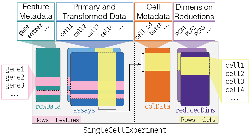
SingleCellExperiment
Load Dataset into R
We next use the read10xCounts function from the DropletUtils package to load the count matrix. This function automatically identifies the count matrix file from CellRanger’s output and reads it in as a SingleCellExperiment object.
fname <- file.path("untar_path", "pbmc4k/raw_gene_bc_matrices/GRCh38")
sce.pbmc <- read10xCounts(fname, col.names=TRUE)
With the data loaded, we can inspect the SCE object to see what information it contains.
class: SingleCellExperiment
dim: 33694 737280
metadata(1): Samples
assays(1): counts
rownames(33694): ENSG00000243485 ENSG00000237613 ... ENSG00000277475
  ENSG00000268674
rowData names(2): ID Symbol
colnames(737280): AAACCTGAGAAACCAT-1 AAACCTGAGAAACCGC-1 ...
  TTTGTCATCTTTAGTC-1 TTTGTCATCTTTCCTC-1
colData names(2): Sample Barcode
reducedDimNames(0):
altExpNames(0):
Questions:
- How many cells are in the SCE object? How many genes?
Removing empty droplets from unfiltered datasets
Droplet-based scRNA-seq methods like 10x increase the throughput of single-cell transcriptomics studies. However, one drawback to droplet-based sequencing is that some of the droplets will not contain a cell and will need to be filtered out computationally. This would be an easy task if empty droplets were truly empty, but in reality these droplets contain “ambient” RNA (free transcripts present in the cell suspension solution that are either actively secreted by cells or released upon cell lysis). These ambient RNAs serve as the base material for reverse transcription and scRNA-seq library preparation, resulting in non-zero counts for cell-less droplets/barcodes.
We can generate a knee plot to visualize the library sizes (i.e. total counts) for each barcode in the dataset. In this plot, high quality barcodes are located on the left and the “knee” represents the inflection point, where to the right barcodes have relatively low counts and may represent empty droplets.
bcrank <- barcodeRanks(counts(sce.pbmc))

# Only showing unique points for plotting speed.
uniq <- !duplicated(bcrank$rank)
plot(bcrank$rank[uniq], bcrank$total[uniq], log="xy",
    xlab="Rank", ylab="Total UMI count", cex.lab=1.2)
Warning in xy.coords(x, y, xlabel, ylabel, log): 1 y value <= 0 omitted from
logarithmic plotabline(h=metadata(bcrank)$inflection, col="darkgreen", lty=2)
abline(h=metadata(bcrank)$knee, col="dodgerblue", lty=2)
legend("bottomleft", legend=c("Inflection", "Knee"),
col=c("darkgreen", "dodgerblue"), lty=2, cex=1.2)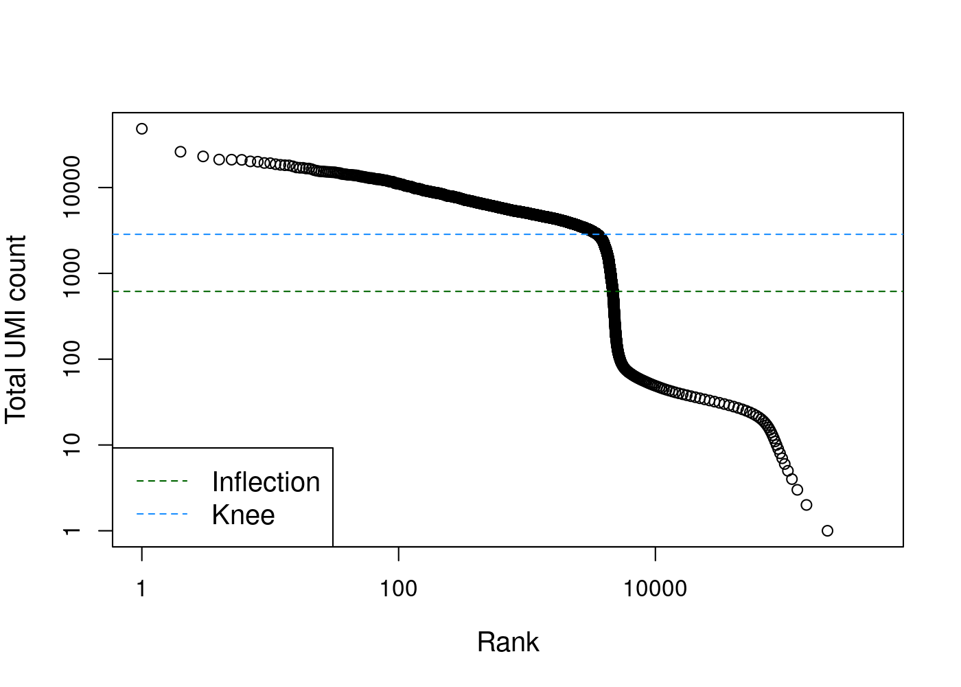
# Total UMI count for each barcode in the PBMC dataset,
# plotted against its rank (in decreasing order of total counts).
# The inferred locations of the inflection and knee points are also shown.
Filtering just by library size may result in eliminating barcodes that contained cells with naturally low expression levels. Luckily, more accurate methods have been developed to filter out cell-less barcodes from droplet-based data. Here we use the emptyDrops method from the DropletUtils package, which estimates the profile of the ambient RNA pool and then tests each barcode for deviations from this profile (Lun et al. 2019).
set.seed(100)
e.out <- emptyDrops(counts(sce.pbmc))
sce.pbmc <- sce.pbmc[,which(e.out$FDR <= 0.001)]
unfiltered <- sce.pbmc
sce.pbmc
class: SingleCellExperiment
dim: 33694 4300
metadata(1): Samples
assays(1): counts
rownames(33694): ENSG00000243485 ENSG00000237613 ... ENSG00000277475
ENSG00000268674
rowData names(2): ID Symbol
colnames(4300): AAACCTGAGAAGGCCT-1 AAACCTGAGACAGACC-1 ...
TTTGTCAGTTAAGACA-1 TTTGTCATCCCAAGAT-1
colData names(2): Sample Barcode
reducedDimNames(0):
altExpNames(0):Questions:
- How many cells are in the SCE object after filtering out empty barcodes?
Annotate genes
Let’s first add row names to rowData and we are going to use gene symbols as the row names. We have to ensure the row name for each gene is unique using the uniquifyFeatureNames function from scater. It will find the duplicated Symbols (some Ensembl IDs share the same gene symbol) and add Ensemble ID as prefix for them so that the rownames are unique.
The PBMC SCE object has the Ensembl ID and the gene symbol for each gene in the rowData. We can add additional annotation information (e.g. chromosome origin) using the annotation database package EnsDb.Hsapiens.v86. Then, to get additional annotations of these genes we can use the IDs as keys to retrieve the information from the database using the mapIds function.
rownames(sce.pbmc) <- uniquifyFeatureNames( ID = rowData(sce.pbmc)$ID,
                                            names = rowData(sce.pbmc)$Symbol)

location <- mapIds(EnsDb.Hsapiens.v86, keys=rowData(sce.pbmc)$ID,
    column="SEQNAME", keytype="GENEID")
Warning: Unable to map 144 of 33694 requested IDs.ENSG00000243485 ENSG00000237613 ENSG00000186092 ENSG00000238009 ENSG00000239945
"1" "1" "1" "1" "1"
ENSG00000239906
"1" Cell-level Quality Control
Calculate cell-level QC metrics
With empty barcodes removed, we can now focus on filtering out low-quality cells (i.e. damaged or dying cells) which might interference with our downstream analysis. It’s common practice to filter cells based on low/high total counts, but we may also want to remove cells with fewer genes expressed. However, for heterogeneous cell populations, like PBMCs, this may remove cell types with naturally low RNA content. So here we will be more relaxed in our filtering and only remove cells with large fraction of read counts from mitochondrial genes. This metric is a proxy for cell damage, where a high proportion of mitochondrial genes would suggest that cytoplasmic mRNA leaked out through a broken membrane, leaving only the mitochondrial mRNAs still in place.
We first calculate QC metrics by perCellQCMetrics function from scater and then filter out the cells with outlying mitochondrial gene proportions.
stats <- perCellQCMetrics(sce.pbmc, subsets=list(Mito=which(location=="MT")))
high.mito <- isOutlier(stats$subsets_Mito_percent, type="higher")
colData(sce.pbmc) <- cbind(colData(sce.pbmc), stats)
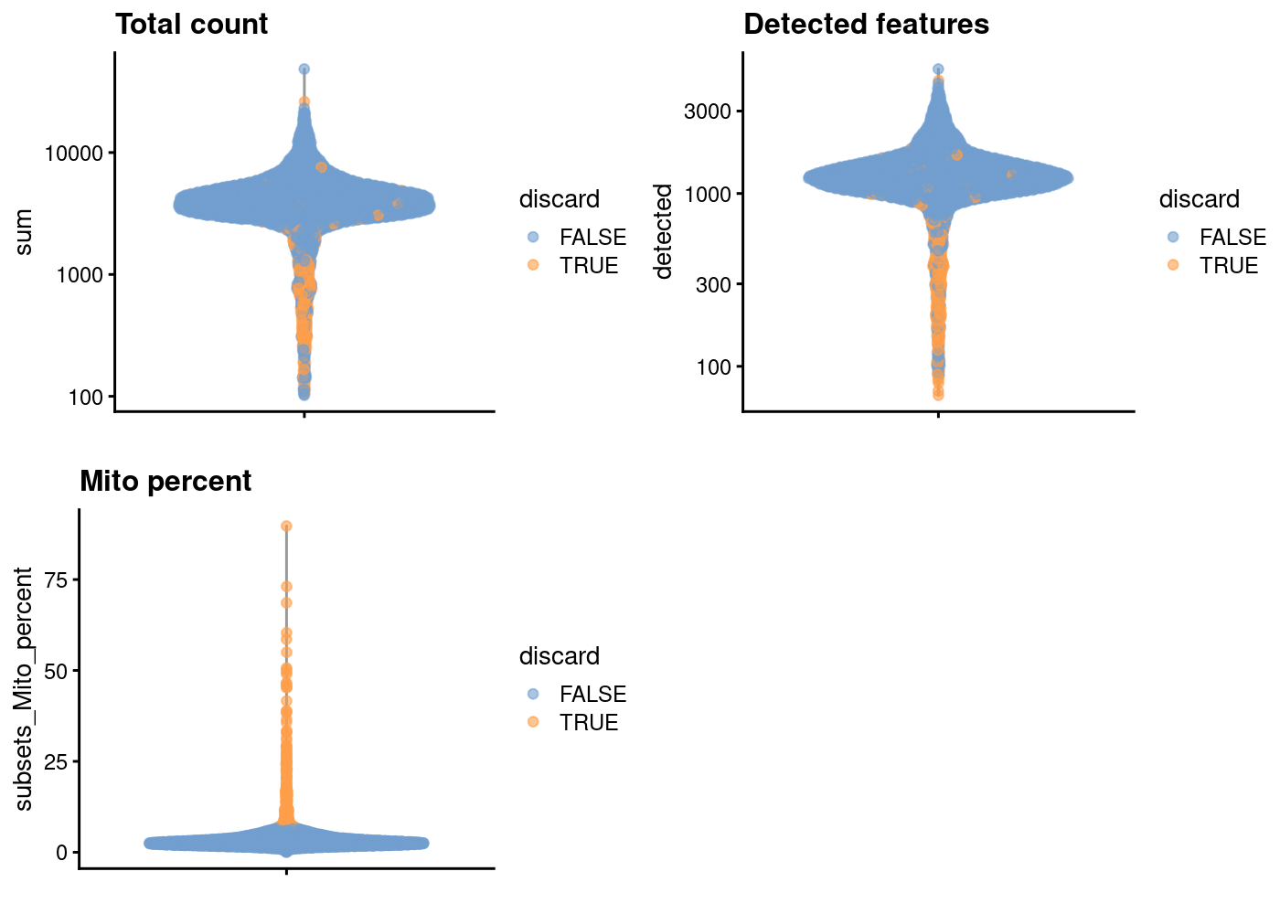
sce.pbmc <- sce.pbmc[,!high.mito]As sanity check, we can look at the library size (i.e. total counts per cell) for cells that will remain after filtering and those that will be removed for having high mitochondrial mRNA proportions. As expected, the cells that will be filtered out (orange) tend to have lower library sizes, but not all cells with low library sizes are removed.
If a large proportion of cells will be removed, then it suggests that the QC metrics we are using for filtering might be correlated with some biological state.
colData(unfiltered) <- cbind(colData(unfiltered), stats)
unfiltered$discard <- high.mito

plotColData(unfiltered, y="sum", colour_by="discard") +
        scale_y_log10() + ggtitle("Total count")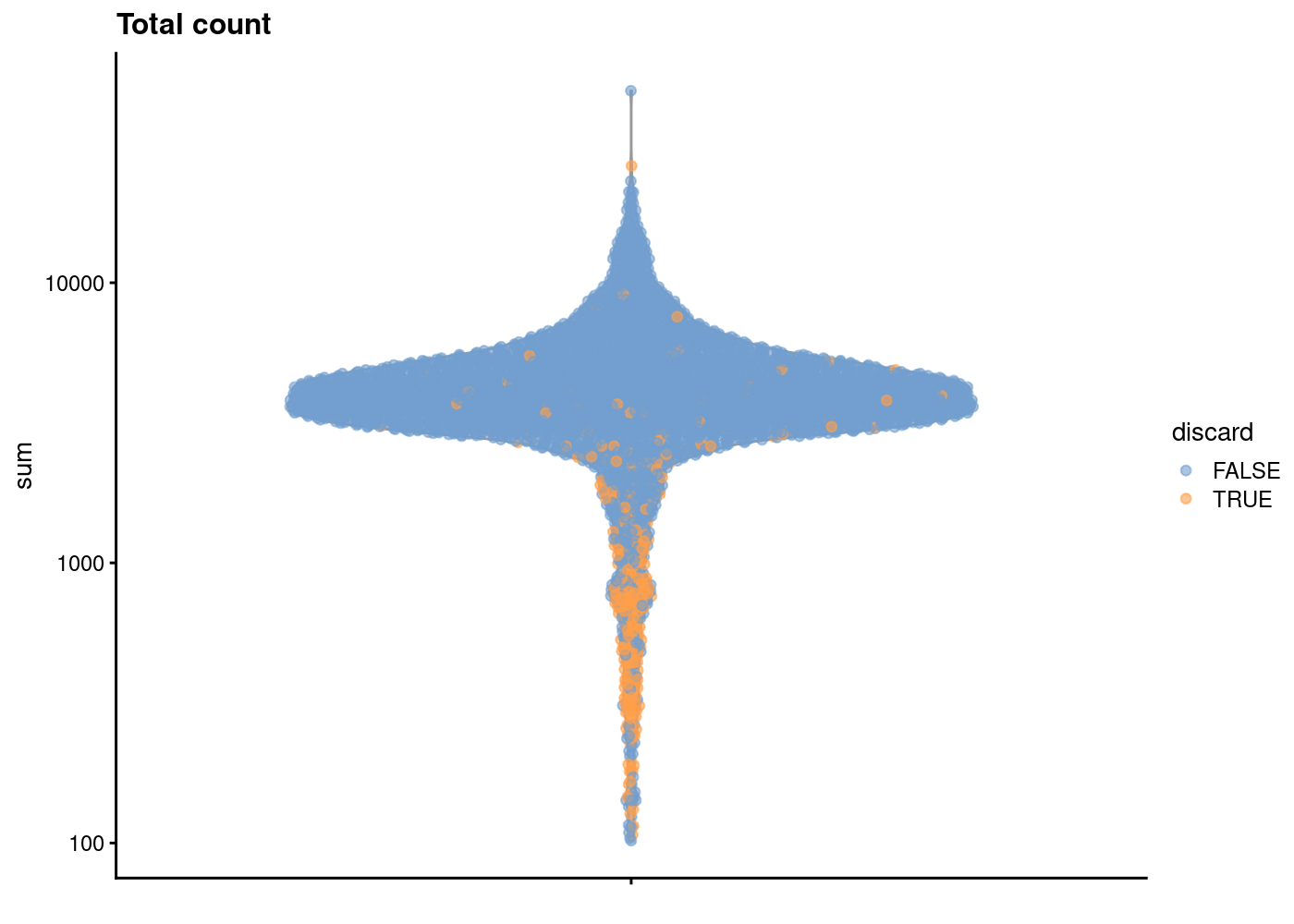
In another view, we plot the subsets_Mito_percent against sum:
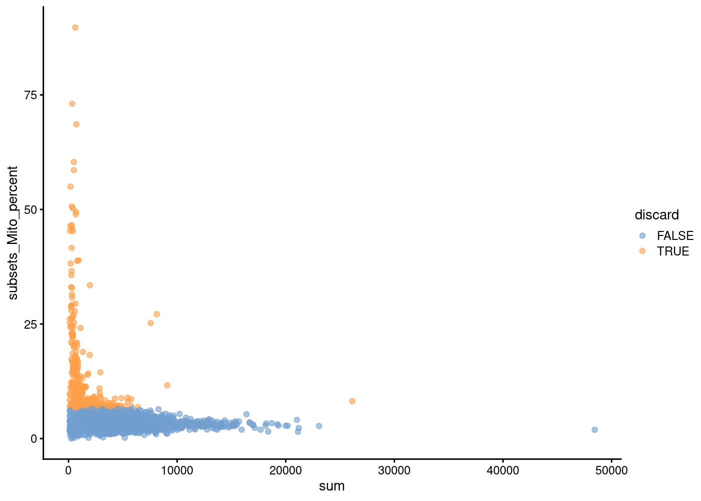 The aim is to confirm that there are no cells with both large total counts and large mitochondrial counts, to ensure that we are not inadvertently removing high-quality cells that happen to be highly metabolically active (e.g., hepatocytes).
Points in the top-right corner might potentially correspond to metabolically active, undamaged cells.
Hands on exercises
—1. Try identifying outlier cells based on low/high total counts—-
—2. Why would be usefule to filter out cells with higher total counts—
—3. Use plotColData to plot other useful cell-level QC metrics (e.g. number of detected features, subsets_Mito_detected) and colour by whether cells would be discarded.—
Hint: you may find the following code helpful.
gridExtra::grid.arrange(
    plotColData(unfiltered, y="sum", colour_by="discard") +
        scale_y_log10() + ggtitle("Total count"),
    plotColData(unfiltered, y="detected", colour_by="discard") +
        scale_y_log10() + ggtitle("Detected features"),
    plotColData(unfiltered, y="subsets_Mito_percent",
        colour_by="discard") + ggtitle("Mito percent"),
    ncol=2
)
Normalisation
Normalisation aims to remove systematic or technical differences (for example, from systematic differences in sequencing coverage across libraries or cells) among cells and samples so they do not interfere with comparisons of the expression profiles.
We are going to use a normalisation method named Normalisation by Deconvolution.
It is a scaling-based procedure that involves dividing all counts for each cell by a cell-specific scaling factor, often called a “size factor”.The size factor for each cell represents the estimate of the relative bias in that cell, so division of its counts by its size factor should remove that bias.
Adapted from bulk RNAseq analysis, we assume the majority of genes between two cells are non-DE (not differential expressed) and the difference among the nonDE genes are used to represent bias that is used to compute an appropriate size factor for its removal.
Given the characteristics of low-counts in single cell dataset, we first pool counts of cells together and estimate a pool-based size factor. The size factor for the pool can be written as a linear equation of the size factors for the cells within the pool. Repeating this process for multiple pools will yield a linear system that can be solved to obtain the size factors for the individual cells, hence deconvolved.
In addition, to avoid pooling too distinct cells together, we first do a quick clustering on the cells, and the normalisation (cell-pooling and deconvolution) is done for each cell cluster separately. (Lun, Bach, and Marioni 2016).
After calculation of the size factors we apply a log transformation to the counts. This transformation is of the form:
\[ \log(\frac{y_{i j}}{s_i} + 1) \]
where \(y_ij\) is the observed count for gene \(j\) in cell \(i\) and \(s_i\) is the calculated size factor for cell \(i\). the division by the size factor removes the scaling bias, as described above, while the \(\log\) transformation helps to stabilize the variance of the counts making downstream visualisation and methods such as PCA more effective. The addition of 1 (sometimes called a pseudocount) is needed as \(\log(0)\) is \(-\infty\) - a value not useful for data analysis.
library(scran)
set.seed(1000)
clusters <- quickCluster(sce.pbmc)
sce.pbmc <- computeSumFactors(sce.pbmc, cluster=clusters)
## normalise using size factor and log-transform them
sce.pbmc <- logNormCounts(sce.pbmc)plot(librarySizeFactors(sce.pbmc), sizeFactors(sce.pbmc), pch=16,
xlab="Library size factors", ylab="Deconvolution factors", log="xy")+abline(a=0,b=1)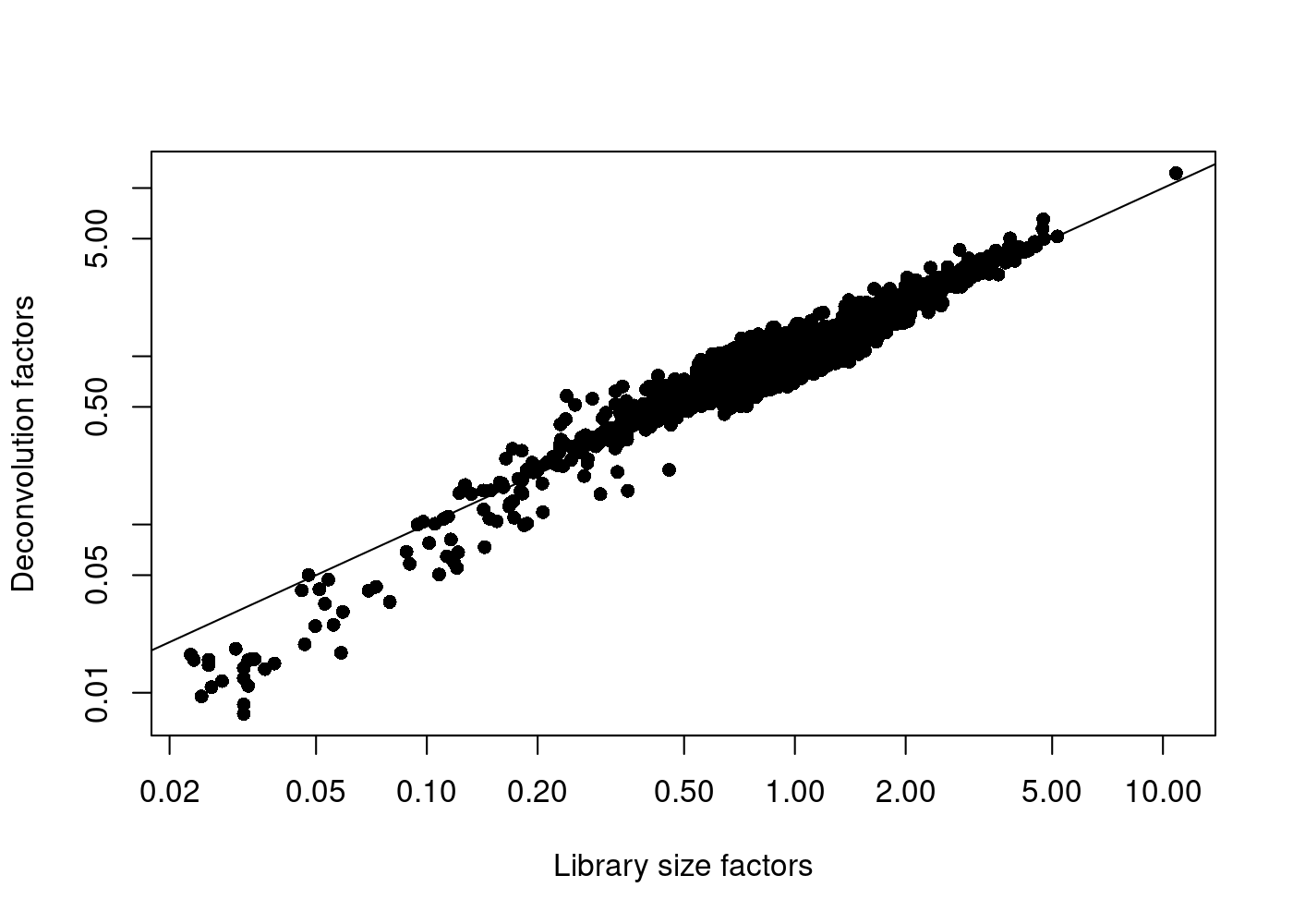
| Version | Author | Date |
|---|---|---|
| 1f42bf1 | rlyu | 2020-11-27 |
integer(0)Alternative normalisation method
Recently, more sophisticated normalisation methods have been developed, for example sctransform (Hafemeister and Satija 2019). The linked webpage contains the instruction for using sctransform for normalisation and feature selection. You can come back to this and try it out later.
— sctransform —
======================================= Break ================================
Variance modeling and feature selection
In this step, we would like to select the features/genes that represent the biological differences among cells while removing noise by other genes. We could simply select the genes with larger variance across the cell population based on the assumption that the most variable genes represent the biological differences rather than just technical noise.
The simplest approach to find such genes is to compute the variance of the log-normalised gene expression values for each gene across all cells. However, the variance of a gene in single-cell RNAseq dataset has a relationship with its mean. log-transformation does not achieve perfect variance stabilisation, which means that the variance of a gene is often driven more by its abundance than its biological heterogeneity.
To deal with this effect, we fit a trend to the variance with respect to the gene’s abundance across all genes to model the mean-variance relationship:
The trend is fitted on simulated Poisson count-derived variances with assumption that the technical component is Poisson-distributed and most genes do not exhibit large biological variability.
plot(dec.pbmc$mean, dec.pbmc$total, pch=16, cex=0.5,
    xlab="Mean of log-expression", ylab="Variance of log-expression")

curfit <- metadata(dec.pbmc)
curve(curfit$trend(x), col='dodgerblue', add=TRUE, lwd=2)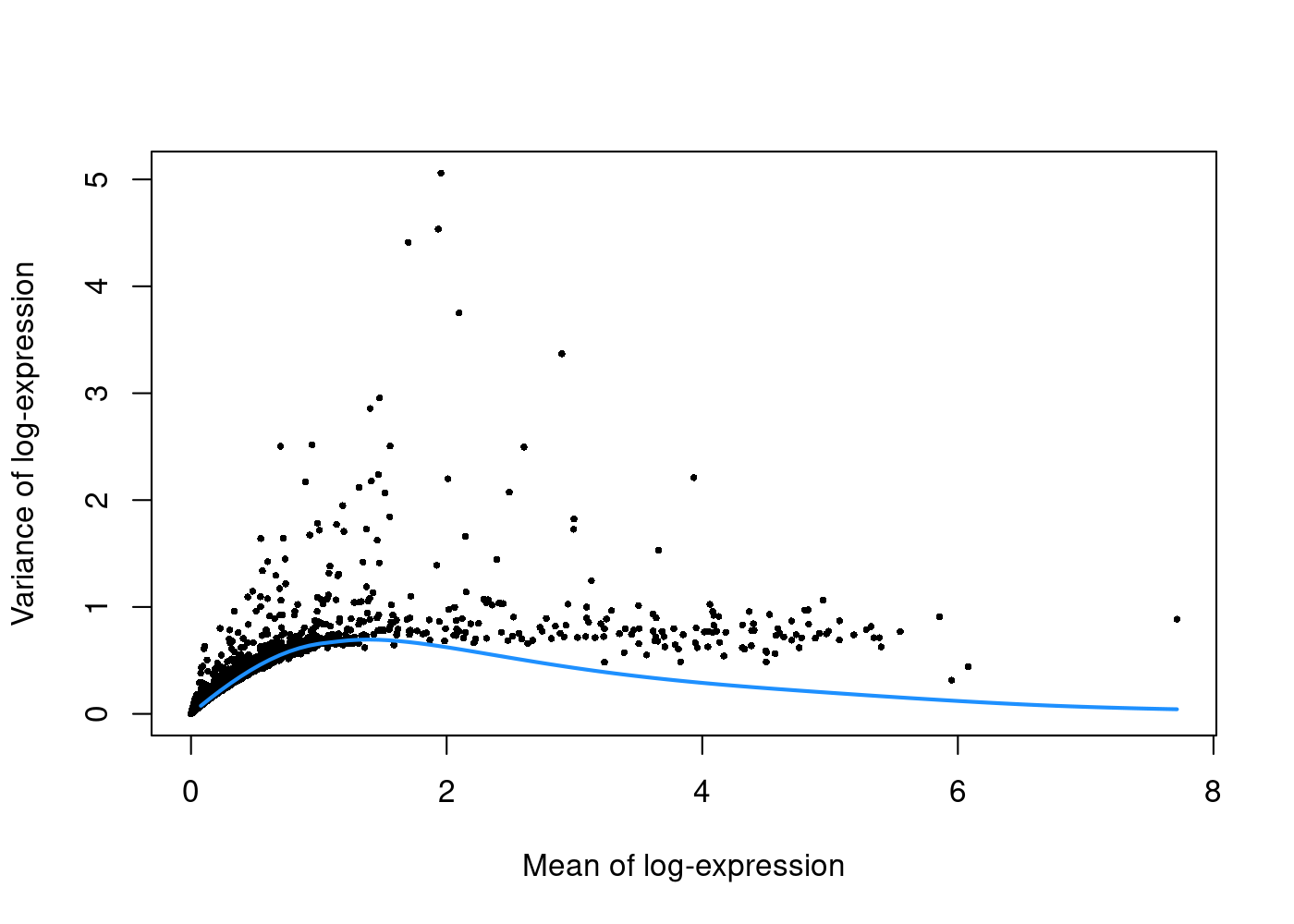
| Version | Author | Date |
|---|---|---|
| 1f42bf1 | rlyu | 2020-11-27 |
Under this assumption, our trend represents an estimate of the technical noise as a function of abundance. The total variance can then be decomposed into technical and biological components.
We can then get the list of highly variable genes after variance decomposition:
About the number of genes to keep, if we believe no more than 5% of genes are differentially expressed across all the cells, we can set the prop to be 5%. In a more heterogeneous cell population, we would raise that number. Here we are using top 10%.
Note that this number selection is actually quite arbitrary. It is recommended to simply pick a value and go ahead with the downstream analysis but with the intention of testing other parameters if needed.
Dimensionality reduction and visualisation
Now we have selected the highly variable genes, we can use these genes’s information to reveal cell population structures in a constructed lower dimensional space. Working with this lower dimensional representation allows for easier exploration and reduces the computational burden of downstream analyses, like clustering. It also helps to reduce noise by averaging information across multiple genes to reveal the structure of the data more precisely.
We first do a PCA (Principal Components Analysis) transformation. By definition, the top PCs capture the dominant factors of heterogeneity in the data set. Thus, we can perform dimensionality reduction by only keeping the top PCs for downstream analyses. The denoisePCA function will automatically choose the number of PCs to keep, using the information returned by the variance decomposition step to remove principal components corresponding to technical noise.
set.seed(10000)
## This function performs a principal components analysis to eliminate random
## technical noise in the data.
sce.pbmc <- denoisePCA(sce.pbmc, subset.row=top.pbmc, technical=dec.pbmc)class: SingleCellExperiment
dim: 33694 3985
metadata(1): Samples
assays(2): counts logcounts
rownames(33694): RP11-34P13.3 FAM138A ... AC213203.1 FAM231B
rowData names(2): ID Symbol
colnames(3985): AAACCTGAGAAGGCCT-1 AAACCTGAGACAGACC-1 ...
TTTGTCAGTTAAGACA-1 TTTGTCATCCCAAGAT-1
colData names(9): Sample Barcode ... total sizeFactor
reducedDimNames(1): PCA
altExpNames(0): PC1 PC2 PC3 PC4 PC5
AAACCTGAGAAGGCCT-1 -16.851284 2.3138660 -1.599521 0.3423342 4.0627139
AAACCTGAGACAGACC-1 -15.534604 6.0260221 -5.066471 0.4879408 1.3860124
AAACCTGAGGCATGGT-1 9.205981 2.0518419 -3.937651 2.6520487 3.1045905
AAACCTGCAAGGTTCT-1 8.528490 -0.2559258 -2.854510 1.0445572 -0.2017011
AAACCTGCAGGCGATA-1 -7.967058 6.0995893 3.391930 -1.8058935 -8.5199572
PC6 PC7 PC8 PC9
AAACCTGAGAAGGCCT-1 1.5483197 1.655729 -0.4606595 -0.6982110
AAACCTGAGACAGACC-1 -1.2024417 2.700262 -0.1728795 0.3074250
AAACCTGAGGCATGGT-1 1.6397698 -2.437645 2.4098404 -0.3039838
AAACCTGCAAGGTTCT-1 1.0021423 1.378933 1.2227933 1.3654361
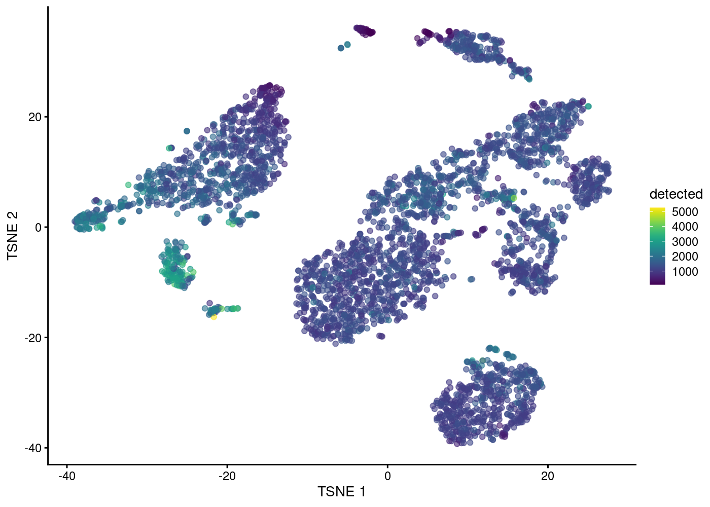
AAACCTGCAGGCGATA-1 0.8870682 -3.583899 0.1580482 5.0634441tSNE (t-stochastic neighbor embedding ) is a popular dimensionality reduction methods for visualising single-cell dataset with functions to run them available in scater. They attempt to find a low-dimensional representation of the data that preserves the distances between each point and its neighbours in the high-dimensional space.
In addition, UMAP (uniform manifold approximation and projection) which is roughly similar to tSNE, is also gaining popularity. They are ways to “visualise” the structure in the dataset and generate nice plots, but shouldn’t be regarded as the real clustering structure.
We actually instruct the function to perform the t-SNE calculations on the top PCs to use the data compaction and noise removal provided by the PCA.
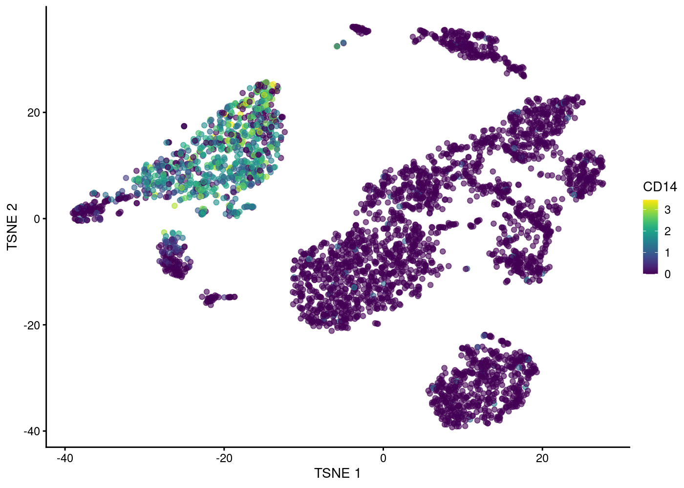
Visualising column data or plotting gene expression in tSNE plot:
| Version | Author | Date |
|---|---|---|
| 1f42bf1 | rlyu | 2020-11-27 |
| Version | Author | Date |
|---|---|---|
| 1f42bf1 | rlyu | 2020-11-27 |
Hexbin plot for overcoming overplotting
Notice that in the 2D plots of single cells, sometimes it can get really “crowded”, especially when the number of cells being plotted is large, and it runs into a over-plotting issue where cells are two close overlaying/blocking To deal with that, we can use the hexbin plots (Freytag and Lister 2020).
schex package provides binning strategies of cells into hexagon cells. Plotting summarized information of all cells in their respective hexagon cells presents information without obstructions.
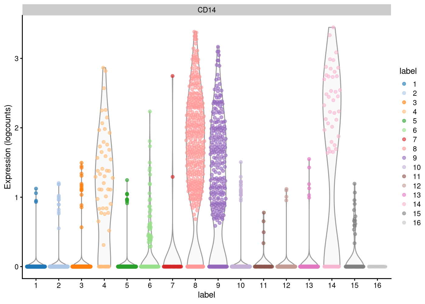
We use the plot_hexbin_feature to plot of feature expression of single cells in bivariate hexagon cells.
pbmc_hex <- schex::make_hexbin(sce.pbmc, 50, dimension_reduction = "TSNE")

plot_hexbin_feature(pbmc_hex,feature="CD14",
                    type = "logcounts",
                    action="median")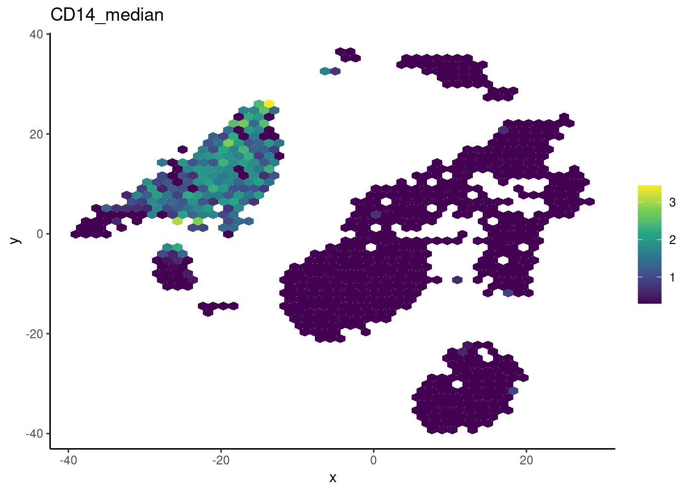
| Version | Author | Date |
|---|---|---|
| bdf4260 | rlyu | 2020-11-25 |
Hands-on practise
—run UMAP and plot—-
—Plot the hexbin plot for UMAP dims—
Clustering
One of the most promising applications of scRNA-seq is de novo discovery and annotation of cell-types based on transcription profiles. We are going to use unsupervised clustering method, that is, we need to identify groups of cells based on the similarities of the transcriptomes without any prior knowledge of the labels.
In scRNAseq analyses, shared K-nearest neighbour graph-based clustering is often applied. Each cell is represented in the graph as a node, and the first step is to find all the KNN (K-neareast neighbours) for each cell by comparing their pair-wise Euclidean distances. After that, the nodes are connected if they have at least one shared nearest neighbors, and weights are also added to the edges by how many shared neighbours they have.
 Once the SNN graph is built, we can then use different algorithms to detect communities/clusters in the graph. Here we use the method called ‘walktrap’ from the igraph package which tries to detect densely connected communities in a graph via random walks.
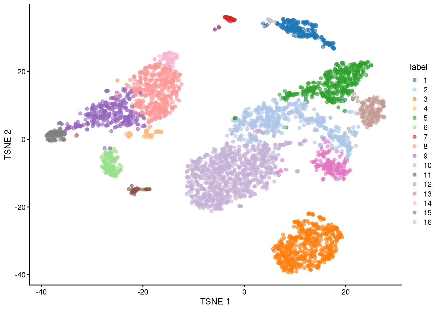
g <- buildSNNGraph(sce.pbmc, k=10, use.dimred = 'PCA')
clust <- igraph::cluster_walktrap(g)$membership
colLabels(sce.pbmc) <- factor(clust)
table(factor(clust))
  1   2   3   4   5   6   7   8   9  10  11  12  13  14  15  16
205 508 541  56 374 125  46 432 302 867  47 155 166  61  84  16
Questions
— Choose different values for k and observe how many clusters you get —
Clustree
clustree can be used to visualise the different clustering results in a tree structure. It helps to visualise how cells move as the clustering resolution changes.
Note, it looks very much like a hierarchical clustering result but it is not.
g <- buildSNNGraph(sce.pbmc, k=5, use.dimred = 'PCA')
k5 <- igraph::cluster_walktrap(g)$membership
g <- buildSNNGraph(sce.pbmc, k=8, use.dimred = 'PCA')
k8 <- igraph::cluster_walktrap(g)$membership

g <- buildSNNGraph(sce.pbmc, k=10, use.dimred = 'PCA')
k10 <- igraph::cluster_walktrap(g)$membership

multipleKResults <- data.frame(k5,k8,k10)
clustree(multipleKResults,prefix = "k",prop_filter =0.05,
         layout="tree")
Warning: The `add` argument of `group_by()` is deprecated as of dplyr 1.0.0.
Please use the `.add` argument instead.
This warning is displayed once every 8 hours.
Call `lifecycle::last_warnings()` to see where this warning was generated.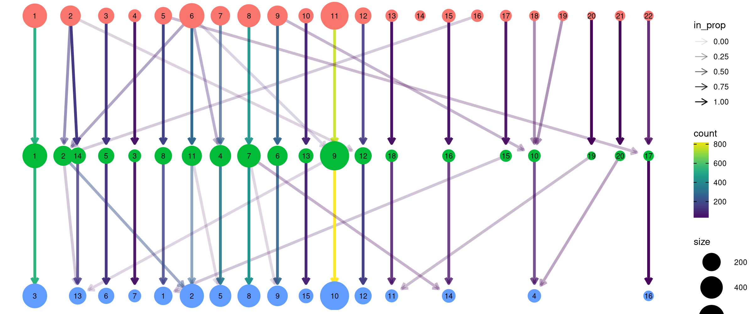
Varying clustering resolutions is an important part of data exploration for scRNAseq. It is challenging to find the best resolution, and you usually need to experiment with different parameters multiple times and try find the proper result.
Marker dection/cluster annotation
To interpret our clustering results, we identify the genes that drive separation between clusters. These marker genes allow us to assign biological meaning to each cluster based on their functional annotation. We demonstrate this approach in the “Manual” annotation.
An alternative way is to use some automatic annotation approach, see the Automatic annotation
“Manual” annotation
findMarkers is done via pair-wise comparisions of all pari-wise combinations of clusters. Each cluster is compared to each of the remaining clusters and up-regulated genes are identified using t-test. The returned results for one cluster (versus any of the remaining clusters) are combined into a single list and the combined.P.values are calculated. One can specifty the pval.type which determines how the DEGs are combined: any, return genes that are determined as up-regulated in any of the comparisons; all, return genes that are determined as up-regulated in all of the comparisons,some is a compromise between any and all.
We examine the markers for cluster 7 and 14 in more detail.
               p.value          FDR summary.logFC
PF4       5.234138e-32 1.763591e-27      6.862880
TMSB4X    4.528537e-25 7.629226e-21      2.902017
TAGLN2    2.312517e-24 2.597265e-20      4.882681
NRGN      1.089643e-22 9.178609e-19      5.008270
SDPR      2.478965e-22 1.670525e-18      5.604447
PPBP      8.573599e-20 4.814647e-16      6.501027
CCL5      5.661811e-19 2.725272e-15      5.307740
GNG11     8.983814e-19 3.593735e-15      5.474025
GPX1      9.599221e-19 3.593735e-15      4.862989
HIST1H2AC 2.850713e-18 9.605193e-15 5.532751 p.value FDR summary.logFC
FTL 7.192158e-64 2.423326e-59 2.145034
LYZ 4.673332e-59 7.873163e-55 5.168217
S100A9 2.387516e-52 2.681499e-48 5.156800
S100A8 1.304486e-43 1.098834e-39 5.553065
RP11-1143G9.4 2.004758e-31 1.350966e-27 3.722163
CTSS 5.705895e-30 3.204241e-26 2.738754
S100A6 2.079948e-29 1.001168e-25 2.477981
LST1 6.177511e-28 2.601813e-24 2.485571
MNDA 2.001599e-25 7.493543e-22 3.049224
DUSP1 2.852678e-20 9.344521e-17 1.705510Question
Now given what we know about the cell types in PBMCs and the marker genes:
— Plot the expression of these marker genes by clusters, and identify what cells types each cluster has —
| Markers | Cell Type |
|---|---|
| IL7R | CD4 T cells |
| CD14, LYZ | CD14+ Monocytes |
| MS4A1 | B cells |
| CD8A | CD8 T cells |
| FCGR3A, MS4A7 | FCGR3A+ Monocytes |
| GNLY , NKG7 | NK cells |
| PPBP | Megakaryocytes |
| FCER1A, CST3 | Dendritic Cells |
| Version | Author | Date |
|---|---|---|
| bdf4260 | rlyu | 2020-11-25 |
Automatic annotation
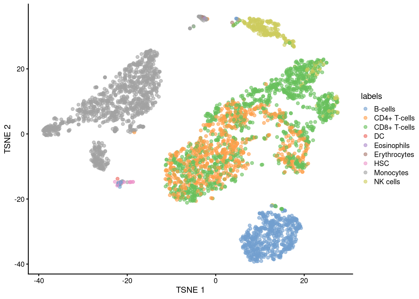
The intuition of automatic annotation is by comparing current dataset with previously annotation reference samples and find the cell type of the most similar/correlated cells. SingleR method (Aran et al. 2019) provides one such option for cell type annotation. This method assigns labels to cells based on the reference samples with the highest Spearman rank correlations, using only the marker genes between pairs of labels to focus on the relevant differences between cell types. It also performs a fine-tuning step for each cell where the correlations are recomputed with just the marker genes for the top-scoring labels. This aims to resolve any ambiguity between those labels by removing noise from irrelevant markers for other labels.
snapshotDate(): 2020-10-02see ?celldex and browseVignettes('celldex') for documentationloading from cachesee ?celldex and browseVignettes('celldex') for documentationloading from cache
     B-cells CD4+ T-cells CD8+ T-cells           DC  Eosinophils Erythrocytes
         549          773         1274            1            1            5
         HSC    Monocytes     NK cells
          14         1117          251
We can check the concordance of the SingleR annotations with our previous clustering result.
                 1   2   3   4   5   6   7   8   9  10  11  12  13  14  15  16
  B-cells        0   0 531   0   0   0   0   0   0   0  15   0   0   0   0   3
  CD4+ T-cells   1 233   0   1   1   0   1   0   0 445   0   0  87   0   0   4
  CD8+ T-cells   6 275   8   0 341   0   0   0   1 422   0 138  79   0   0   4
  DC             0   0   0   0   0   0   0   0   0   0   1   0   0   0   0   0
  Eosinophils    0   0   0   0   0   0   1   0   0   0   0   0   0   0   0   0
  Erythrocytes   1   0   0   0   0   0   4   0   0   0   0   0   0   0   0   0
  HSC            0   0   0   0   0   0   0   0   0   0  14   0   0   0   0   0
  Monocytes      0   0   0  55   0 125  40 432 301   0  17   0   0  61  84   2
  NK cells     197   0   2   0  32   0   0   0   0   0   0  17   0   0   0   3
Cell type annotation plots
Now with the labels learned from SingleR methods, we can visualise them in a tSNE plot.
| Version | Author | Date |
|---|---|---|
| 1f42bf1 | rlyu | 2020-11-27 |
Further exploration
The scRNAseq package provides convenient access to a list of publicly available data sets in the form of SingleCellExperiment objects. You can choose one of them to practice these steps we introduced above.
More resources:
https://biocellgen-public.svi.edu.au/mig_2019_scrnaseq-workshop/public/index.html
SessionInfo
R version 4.0.3 (2020-10-10)
Platform: x86_64-pc-linux-gnu (64-bit)
Running under: Red Hat Enterprise Linux

Matrix products: default
BLAS/LAPACK: /usr/lib64/libopenblasp-r0.3.3.so

locale:
 [1] LC_CTYPE=en_AU.UTF-8       LC_NUMERIC=C
 [3] LC_TIME=en_AU.UTF-8        LC_COLLATE=en_AU.UTF-8
 [5] LC_MONETARY=en_AU.UTF-8    LC_MESSAGES=en_AU.UTF-8
 [7] LC_PAPER=en_AU.UTF-8       LC_NAME=C
 [9] LC_ADDRESS=C               LC_TELEPHONE=C
[11] LC_MEASUREMENT=en_AU.UTF-8 LC_IDENTIFICATION=C

attached base packages:
[1] parallel  stats4    stats     graphics  grDevices utils     datasets
[8] methods   base

other attached packages:
 [1] gridExtra_2.3               SingleR_1.4.0
 [3] celldex_1.0.0               schex_1.4.0
 [5] shiny_1.5.0                 Seurat_3.2.2
 [7] EnsDb.Hsapiens.v86_2.99.0   ensembldb_2.14.0
 [9] AnnotationFilter_1.14.0     GenomicFeatures_1.42.0
[11] AnnotationDbi_1.52.0        DropletUtils_1.10.0
[13] BiocFileCache_1.14.0        dbplyr_2.0.0
[15] Rtsne_0.15                  BiocSingular_1.6.0
[17] clustree_0.4.3              ggraph_2.0.3
[19] scran_1.18.0                scater_1.18.0
[21] ggplot2_3.3.2               scRNAseq_2.3.17
[23] SingleCellExperiment_1.12.0 SummarizedExperiment_1.20.0
[25] Biobase_2.50.0              GenomicRanges_1.42.0
[27] GenomeInfoDb_1.26.0         IRanges_2.24.0
[29] S4Vectors_0.28.0            BiocGenerics_0.36.0
[31] MatrixGenerics_1.2.0        matrixStats_0.57.0

loaded via a namespace (and not attached):
  [1] rappdirs_0.3.1                rtracklayer_1.50.0
  [3] R.methodsS3_1.8.1             tidyr_1.1.2
  [5] bit64_4.0.5                   knitr_1.30
  [7] irlba_2.3.3                   DelayedArray_0.16.0
  [9] R.utils_2.10.1                data.table_1.13.2
 [11] rpart_4.1-15                  RCurl_1.98-1.2
 [13] generics_0.1.0                cowplot_1.1.0
 [15] RSQLite_2.2.1                 RANN_2.6.1
 [17] future_1.20.1                 bit_4.0.4
 [19] spatstat.data_1.4-3           xml2_1.3.2
 [21] httpuv_1.5.4                  assertthat_0.2.1
 [23] viridis_0.5.1                 xfun_0.19
 [25] hms_0.5.3                     evaluate_0.14
 [27] promises_1.1.1                progress_1.2.2
 [29] igraph_1.2.6                  DBI_1.1.0
 [31] htmlwidgets_1.5.2             purrr_0.3.4
 [33] ellipsis_0.3.1                dplyr_1.0.2
 [35] backports_1.2.0               biomaRt_2.46.0
 [37] deldir_0.2-2                  sparseMatrixStats_1.2.0
 [39] vctrs_0.3.4                   ROCR_1.0-11
 [41] entropy_1.2.1                 abind_1.4-5
 [43] withr_2.3.0                   ggforce_0.3.2
 [45] checkmate_2.0.0               sctransform_0.3.1
 [47] GenomicAlignments_1.26.0      prettyunits_1.1.1
 [49] goftest_1.2-2                 cluster_2.1.0
 [51] ExperimentHub_1.16.0          lazyeval_0.2.2
 [53] crayon_1.3.4                  labeling_0.4.2
 [55] edgeR_3.32.0                  pkgconfig_2.0.3
 [57] tweenr_1.0.1                  nlme_3.1-149
 [59] vipor_0.4.5                   ProtGenerics_1.22.0
 [61] rlang_0.4.8                   globals_0.13.1
 [63] lifecycle_0.2.0               miniUI_0.1.1.1
 [65] rsvd_1.0.3                    AnnotationHub_2.22.0
 [67] rprojroot_1.3-2               polyclip_1.10-0
 [69] lmtest_0.9-38                 Matrix_1.2-18
 [71] Rhdf5lib_1.12.0               zoo_1.8-8
 [73] beeswarm_0.2.3                whisker_0.4
 [75] ggridges_0.5.2                png_0.1-7
 [77] viridisLite_0.3.0             bitops_1.0-6
 [79] R.oo_1.24.0                   KernSmooth_2.23-17
 [81] rhdf5filters_1.2.0            Biostrings_2.58.0
 [83] blob_1.2.1                    DelayedMatrixStats_1.12.0
 [85] workflowr_1.6.2               stringr_1.4.0
 [87] parallelly_1.21.0             beachmat_2.6.0
 [89] scales_1.1.1                  hexbin_1.28.1
 [91] memoise_1.1.0                 magrittr_1.5
 [93] plyr_1.8.6                    ica_1.0-2
 [95] zlibbioc_1.36.0               compiler_4.0.3
 [97] concaveman_1.1.0              dqrng_0.2.1
 [99] RColorBrewer_1.1-2            fitdistrplus_1.1-1
[101] Rsamtools_2.6.0               XVector_0.30.0
[103] listenv_0.8.0                 patchwork_1.0.1
[105] pbapply_1.4-3                 mgcv_1.8-33
[107] MASS_7.3-53                   tidyselect_1.1.0
[109] stringi_1.5.3                 yaml_2.2.1
[111] askpass_1.1                   locfit_1.5-9.4
[113] ggrepel_0.8.2                 grid_4.0.3
[115] tools_4.0.3                   future.apply_1.6.0
[117] rstudioapi_0.11               bluster_1.0.0
[119] git2r_0.27.1                  farver_2.0.3
[121] digest_0.6.27                 BiocManager_1.30.10
[123] Rcpp_1.0.5                    scuttle_1.0.0
[125] BiocVersion_3.12.0            later_1.1.0.1
[127] RcppAnnoy_0.0.16              httr_1.4.2
[129] colorspace_1.4-1              tensor_1.5
[131] XML_3.99-0.5                  fs_1.5.0
[133] reticulate_1.18               splines_4.0.3
[135] uwot_0.1.8                    statmod_1.4.35
[137] spatstat.utils_1.17-0         graphlayouts_0.7.1
[139] plotly_4.9.2.1                xtable_1.8-4
[141] jsonlite_1.7.1                spatstat_1.64-1
[143] tidygraph_1.2.0               R6_2.5.0
[145] pillar_1.4.6                  htmltools_0.5.0
[147] mime_0.9                      glue_1.4.2
[149] fastmap_1.0.1                 BiocParallel_1.24.0
[151] BiocNeighbors_1.8.0           interactiveDisplayBase_1.28.0
[153] codetools_0.2-16              lattice_0.20-41
[155] tibble_3.0.4                  curl_4.3
[157] ggbeeswarm_0.6.0              leiden_0.3.4
[159] openssl_1.4.3                 survival_3.2-7
[161] limma_3.46.0                  rmarkdown_2.5
[163] munsell_0.5.0                 rhdf5_2.34.0
[165] GenomeInfoDbData_1.2.4        HDF5Array_1.18.0
[167] reshape2_1.4.4                gtable_0.3.0
References
Amezquita, Robert A, Aaron T L Lun, Etienne Becht, Vince J Carey, Lindsay N Carpp, Ludwig Geistlinger, Federico Martini, et al. 2019. “Orchestrating Single-Cell Analysis with Bioconductor.” Nat. Methods, December.
Aran, Dvir, Agnieszka P Looney, Leqian Liu, Esther Wu, Valerie Fong, Austin Hsu, Suzanna Chak, et al. 2019. “Reference-Based Analysis of Lung Single-Cell Sequencing Reveals a Transitional Profibrotic Macrophage.” Nat. Immunol. 20 (2): 163–72.
Freytag, Saskia, and Ryan Lister. 2020. “Schex Avoids Overplotting for Large Single-Cell RNA-sequencing Datasets.” Bioinformatics 36 (7): 2291–2.
Hafemeister, Christoph, and Rahul Satija. 2019. “Normalization and Variance Stabilization of Single-Cell RNA-seq Data Using Regularized Negative Binomial Regression.” Genome Biol. 20 (1): 296.
Lun, Aaron T L, Karsten Bach, and John C Marioni. 2016. “Pooling Across Cells to Normalize Single-Cell RNA Sequencing Data with Many Zero Counts.” Genome Biol. 17 (April): 75.
Lun, Aaron T L, Samantha Riesenfeld, Tallulah Andrews, The Phuong Dao, Tomas Gomes, participants in the 1st Human Cell Atlas Jamboree, and John C Marioni. 2019. “EmptyDrops: Distinguishing Cells from Empty Droplets in Droplet-Based Single-Cell RNA Sequencing Data.” Genome Biol. 20 (1): 63.
Zheng, Grace X Y, Jessica M Terry, Phillip Belgrader, Paul Ryvkin, Zachary W Bent, Ryan Wilson, Solongo B Ziraldo, et al. 2017. “Massively Parallel Digital Transcriptional Profiling of Single Cells.” Nat. Commun. 8 (January): 14049.
Registered S3 method overwritten by 'cli':
  method     from
  print.boxx spatstat
─ Session info ───────────────────────────────────────────────────────────────
setting value
version R version 4.0.3 (2020-10-10)
os Red Hat Enterprise Linux
system x86_64, linux-gnu
ui X11
language (EN)
collate en_AU.UTF-8
ctype en_AU.UTF-8
tz Australia/Melbourne
date 2020-11-30
─ Packages ───────────────────────────────────────────────────────────────────
package * version date lib source
abind 1.4-5 2016-07-21 [1] CRAN (R 4.0.2)
AnnotationDbi * 1.52.0 2020-10-27 [1] Bioconductor
AnnotationFilter * 1.14.0 2020-10-27 [1] Bioconductor
AnnotationHub 2.22.0 2020-10-27 [1] Bioconductor
askpass 1.1 2019-01-13 [1] CRAN (R 4.0.2)
assertthat 0.2.1 2019-03-21 [1] CRAN (R 4.0.2)
backports 1.2.0 2020-11-02 [1] CRAN (R 4.0.2)
beachmat 2.6.0 2020-10-27 [1] Bioconductor
beeswarm 0.2.3 2016-04-25 [1] CRAN (R 4.0.2)
Biobase * 2.50.0 2020-10-27 [1] Bioconductor
BiocFileCache * 1.14.0 2020-10-27 [1] Bioconductor
BiocGenerics * 0.36.0 2020-10-27 [1] Bioconductor
BiocManager 1.30.10 2019-11-16 [1] CRAN (R 4.0.2)
BiocNeighbors 1.8.0 2020-10-27 [1] Bioconductor
BiocParallel 1.24.0 2020-10-27 [1] Bioconductor
BiocSingular * 1.6.0 2020-10-27 [1] Bioconductor
BiocVersion 3.12.0 2020-04-27 [1] Bioconductor
biomaRt 2.46.0 2020-10-27 [1] Bioconductor
Biostrings 2.58.0 2020-10-27 [1] Bioconductor
bit 4.0.4 2020-08-04 [1] CRAN (R 4.0.2)
bit64 4.0.5 2020-08-30 [1] CRAN (R 4.0.2)
bitops 1.0-6 2013-08-17 [1] CRAN (R 4.0.2)
blob 1.2.1 2020-01-20 [1] CRAN (R 4.0.2)
bluster 1.0.0 2020-10-27 [1] Bioconductor
callr 3.5.1 2020-10-13 [1] CRAN (R 4.0.2)
celldex * 1.0.0 2020-10-29 [1] Bioconductor
checkmate 2.0.0 2020-02-06 [1] CRAN (R 4.0.2)
cli 2.1.0 2020-10-12 [1] CRAN (R 4.0.2)
cluster 2.1.0 2019-06-19 [2] CRAN (R 4.0.3)
clustree * 0.4.3 2020-06-14 [1] CRAN (R 4.0.2)
codetools 0.2-16 2018-12-24 [2] CRAN (R 4.0.3)
colorspace 1.4-1 2019-03-18 [1] CRAN (R 4.0.2)
concaveman 1.1.0 2020-05-11 [1] CRAN (R 4.0.2)
cowplot 1.1.0 2020-09-08 [1] CRAN (R 4.0.2)
crayon 1.3.4 2017-09-16 [1] CRAN (R 4.0.2)
curl 4.3 2019-12-02 [1] CRAN (R 4.0.2)
data.table 1.13.2 2020-10-19 [1] CRAN (R 4.0.2)
DBI 1.1.0 2019-12-15 [1] CRAN (R 4.0.2)
dbplyr * 2.0.0 2020-11-03 [1] CRAN (R 4.0.2)
DelayedArray 0.16.0 2020-10-27 [1] Bioconductor
DelayedMatrixStats 1.12.0 2020-10-27 [1] Bioconductor
deldir 0.2-2 2020-11-05 [1] CRAN (R 4.0.2)
desc 1.2.0 2018-05-01 [1] CRAN (R 4.0.2)
devtools 2.3.2 2020-09-18 [1] CRAN (R 4.0.2)
digest 0.6.27 2020-10-24 [1] CRAN (R 4.0.2)
dplyr 1.0.2 2020-08-18 [1] CRAN (R 4.0.2)
dqrng 0.2.1 2019-05-17 [1] CRAN (R 4.0.2)
DropletUtils * 1.10.0 2020-10-27 [1] Bioconductor
edgeR 3.32.0 2020-10-27 [1] Bioconductor
ellipsis 0.3.1 2020-05-15 [1] CRAN (R 4.0.2)
EnsDb.Hsapiens.v86 * 2.99.0 2020-11-05 [1] Bioconductor
ensembldb * 2.14.0 2020-10-27 [1] Bioconductor
entropy 1.2.1 2014-11-14 [1] CRAN (R 4.0.2)
evaluate 0.14 2019-05-28 [1] CRAN (R 4.0.2)
ExperimentHub 1.16.0 2020-10-27 [1] Bioconductor
fansi 0.4.1 2020-01-08 [1] CRAN (R 4.0.2)
farver 2.0.3 2020-01-16 [1] CRAN (R 4.0.2)
fastmap 1.0.1 2019-10-08 [1] CRAN (R 4.0.2)
fitdistrplus 1.1-1 2020-05-19 [1] CRAN (R 4.0.2)
fs 1.5.0 2020-07-31 [1] CRAN (R 4.0.2)
future 1.20.1 2020-11-03 [1] CRAN (R 4.0.2)
future.apply 1.6.0 2020-07-01 [1] CRAN (R 4.0.2)
generics 0.1.0 2020-10-31 [1] CRAN (R 4.0.2)
GenomeInfoDb * 1.26.0 2020-10-27 [1] Bioconductor
GenomeInfoDbData 1.2.4 2020-11-04 [1] Bioconductor
GenomicAlignments 1.26.0 2020-10-27 [1] Bioconductor
GenomicFeatures * 1.42.0 2020-10-27 [1] Bioconductor
GenomicRanges * 1.42.0 2020-10-27 [1] Bioconductor
ggbeeswarm 0.6.0 2017-08-07 [1] CRAN (R 4.0.2)
ggforce 0.3.2 2020-06-23 [1] CRAN (R 4.0.2)
ggplot2 * 3.3.2 2020-06-19 [1] CRAN (R 4.0.2)
ggraph * 2.0.3 2020-05-20 [1] CRAN (R 4.0.2)
ggrepel 0.8.2 2020-03-08 [1] CRAN (R 4.0.2)
ggridges 0.5.2 2020-01-12 [1] CRAN (R 4.0.2)
git2r 0.27.1 2020-05-03 [1] CRAN (R 4.0.2)
globals 0.13.1 2020-10-11 [1] CRAN (R 4.0.2)
glue 1.4.2 2020-08-27 [1] CRAN (R 4.0.2)
goftest 1.2-2 2019-12-02 [1] CRAN (R 4.0.2)
graphlayouts 0.7.1 2020-10-26 [1] CRAN (R 4.0.2)
gridExtra * 2.3 2017-09-09 [1] CRAN (R 4.0.2)
gtable 0.3.0 2019-03-25 [1] CRAN (R 4.0.2)
HDF5Array 1.18.0 2020-10-27 [1] Bioconductor
hexbin 1.28.1 2020-02-03 [1] CRAN (R 4.0.2)
hms 0.5.3 2020-01-08 [1] CRAN (R 4.0.2)
htmltools 0.5.0 2020-06-16 [1] CRAN (R 4.0.2)
htmlwidgets 1.5.2 2020-10-03 [1] CRAN (R 4.0.2)
httpuv 1.5.4 2020-06-06 [1] CRAN (R 4.0.2)
httr 1.4.2 2020-07-20 [1] CRAN (R 4.0.2)
ica 1.0-2 2018-05-24 [1] CRAN (R 4.0.2)
igraph 1.2.6 2020-10-06 [1] CRAN (R 4.0.2)
interactiveDisplayBase 1.28.0 2020-10-27 [1] Bioconductor
IRanges * 2.24.0 2020-10-27 [1] Bioconductor
irlba 2.3.3 2019-02-05 [1] CRAN (R 4.0.2)
jsonlite 1.7.1 2020-09-07 [1] CRAN (R 4.0.2)
KernSmooth 2.23-17 2020-04-26 [2] CRAN (R 4.0.3)
knitr 1.30 2020-09-22 [1] CRAN (R 4.0.2)
labeling 0.4.2 2020-10-20 [1] CRAN (R 4.0.2)
later 1.1.0.1 2020-06-05 [1] CRAN (R 4.0.2)
lattice 0.20-41 2020-04-02 [2] CRAN (R 4.0.3)
lazyeval 0.2.2 2019-03-15 [1] CRAN (R 4.0.2)
leiden 0.3.4 2020-10-29 [1] CRAN (R 4.0.2)
lifecycle 0.2.0 2020-03-06 [1] CRAN (R 4.0.2)
limma 3.46.0 2020-10-27 [1] Bioconductor
listenv 0.8.0 2019-12-05 [1] CRAN (R 4.0.2)
lmtest 0.9-38 2020-09-09 [1] CRAN (R 4.0.2)
locfit 1.5-9.4 2020-03-25 [1] CRAN (R 4.0.2)
magrittr 1.5 2014-11-22 [1] CRAN (R 4.0.2)
MASS 7.3-53 2020-09-09 [2] CRAN (R 4.0.3)
Matrix 1.2-18 2019-11-27 [2] CRAN (R 4.0.3)
MatrixGenerics * 1.2.0 2020-10-27 [1] Bioconductor
matrixStats * 0.57.0 2020-09-25 [1] CRAN (R 4.0.2)
memoise 1.1.0 2017-04-21 [1] CRAN (R 4.0.2)
mgcv 1.8-33 2020-08-27 [2] CRAN (R 4.0.3)
mime 0.9 2020-02-04 [1] CRAN (R 4.0.2)
miniUI 0.1.1.1 2018-05-18 [1] CRAN (R 4.0.2)
munsell 0.5.0 2018-06-12 [1] CRAN (R 4.0.2)
nlme 3.1-149 2020-08-23 [2] CRAN (R 4.0.3)
openssl 1.4.3 2020-09-18 [1] CRAN (R 4.0.2)
parallelly 1.21.0 2020-10-27 [1] CRAN (R 4.0.2)
patchwork 1.0.1 2020-06-22 [1] CRAN (R 4.0.2)
pbapply 1.4-3 2020-08-18 [1] CRAN (R 4.0.2)
pillar 1.4.6 2020-07-10 [1] CRAN (R 4.0.2)
pkgbuild 1.1.0 2020-07-13 [1] CRAN (R 4.0.2)
pkgconfig 2.0.3 2019-09-22 [1] CRAN (R 4.0.2)
pkgload 1.1.0 2020-05-29 [1] CRAN (R 4.0.2)
plotly 4.9.2.1 2020-04-04 [1] CRAN (R 4.0.2)
plyr 1.8.6 2020-03-03 [1] CRAN (R 4.0.2)
png 0.1-7 2013-12-03 [1] CRAN (R 4.0.2)
polyclip 1.10-0 2019-03-14 [1] CRAN (R 4.0.2)
prettyunits 1.1.1 2020-01-24 [1] CRAN (R 4.0.2)
processx 3.4.4 2020-09-03 [1] CRAN (R 4.0.2)
progress 1.2.2 2019-05-16 [1] CRAN (R 4.0.2)
promises 1.1.1 2020-06-09 [1] CRAN (R 4.0.2)
ProtGenerics 1.22.0 2020-10-27 [1] Bioconductor
ps 1.4.0 2020-10-07 [1] CRAN (R 4.0.2)
purrr 0.3.4 2020-04-17 [1] CRAN (R 4.0.2)
R.methodsS3 1.8.1 2020-08-26 [1] CRAN (R 4.0.2)
R.oo 1.24.0 2020-08-26 [1] CRAN (R 4.0.2)
R.utils 2.10.1 2020-08-26 [1] CRAN (R 4.0.2)
R6 2.5.0 2020-10-28 [1] CRAN (R 4.0.2)
RANN 2.6.1 2019-01-08 [1] CRAN (R 4.0.2)
rappdirs 0.3.1 2016-03-28 [1] CRAN (R 4.0.2)
RColorBrewer 1.1-2 2014-12-07 [1] CRAN (R 4.0.2)
Rcpp 1.0.5 2020-07-06 [1] CRAN (R 4.0.2)
RcppAnnoy 0.0.16 2020-03-08 [1] CRAN (R 4.0.2)
RCurl 1.98-1.2 2020-04-18 [1] CRAN (R 4.0.2)
remotes 2.2.0 2020-07-21 [1] CRAN (R 4.0.2)
reshape2 1.4.4 2020-04-09 [1] CRAN (R 4.0.2)
reticulate 1.18 2020-10-25 [1] CRAN (R 4.0.2)
rhdf5 2.34.0 2020-10-27 [1] Bioconductor
rhdf5filters 1.2.0 2020-10-27 [1] Bioconductor
Rhdf5lib 1.12.0 2020-10-27 [1] Bioconductor
rlang 0.4.8 2020-10-08 [1] CRAN (R 4.0.2)
rmarkdown 2.5 2020-10-21 [1] CRAN (R 4.0.2)
ROCR 1.0-11 2020-05-02 [1] CRAN (R 4.0.2)
rpart 4.1-15 2019-04-12 [2] CRAN (R 4.0.3)
rprojroot 1.3-2 2018-01-03 [1] CRAN (R 4.0.2)
Rsamtools 2.6.0 2020-10-27 [1] Bioconductor
RSQLite 2.2.1 2020-09-30 [1] CRAN (R 4.0.2)
rstudioapi 0.11 2020-02-07 [1] CRAN (R 4.0.2)
rsvd 1.0.3 2020-02-17 [1] CRAN (R 4.0.2)
rtracklayer 1.50.0 2020-10-27 [1] Bioconductor
Rtsne * 0.15 2018-11-10 [1] CRAN (R 4.0.2)
S4Vectors * 0.28.0 2020-10-27 [1] Bioconductor
scales 1.1.1 2020-05-11 [1] CRAN (R 4.0.2)
scater * 1.18.0 2020-10-27 [1] Bioconductor
schex * 1.4.0 2020-10-27 [1] Bioconductor
scran * 1.18.0 2020-10-27 [1] Bioconductor
scRNAseq * 2.3.17 2020-10-19 [1] Bioconductor
sctransform 0.3.1 2020-10-08 [1] CRAN (R 4.0.2)
scuttle 1.0.0 2020-10-27 [1] Bioconductor
sessioninfo 1.1.1 2018-11-05 [1] CRAN (R 4.0.2)
Seurat * 3.2.2 2020-09-26 [1] CRAN (R 4.0.2)
shiny * 1.5.0 2020-06-23 [1] CRAN (R 4.0.2)
SingleCellExperiment * 1.12.0 2020-10-27 [1] Bioconductor
SingleR * 1.4.0 2020-10-27 [1] Bioconductor
sparseMatrixStats 1.2.0 2020-10-27 [1] Bioconductor
spatstat 1.64-1 2020-05-12 [1] CRAN (R 4.0.2)
spatstat.data 1.4-3 2020-01-26 [1] CRAN (R 4.0.2)
spatstat.utils 1.17-0 2020-02-07 [1] CRAN (R 4.0.2)
statmod 1.4.35 2020-10-19 [1] CRAN (R 4.0.2)
stringi 1.5.3 2020-09-09 [1] CRAN (R 4.0.2)
stringr 1.4.0 2019-02-10 [1] CRAN (R 4.0.2)
SummarizedExperiment * 1.20.0 2020-10-27 [1] Bioconductor
survival 3.2-7 2020-09-28 [2] CRAN (R 4.0.3)
tensor 1.5 2012-05-05 [1] CRAN (R 4.0.2)
testthat 3.0.0 2020-10-31 [1] CRAN (R 4.0.2)
tibble 3.0.4 2020-10-12 [1] CRAN (R 4.0.2)
tidygraph 1.2.0 2020-05-12 [1] CRAN (R 4.0.2)
tidyr 1.1.2 2020-08-27 [1] CRAN (R 4.0.2)
tidyselect 1.1.0 2020-05-11 [1] CRAN (R 4.0.2)
tweenr 1.0.1 2018-12-14 [1] CRAN (R 4.0.2)
usethis 1.6.3 2020-09-17 [1] CRAN (R 4.0.2)
uwot 0.1.8 2020-03-16 [1] CRAN (R 4.0.2)
vctrs 0.3.4 2020-08-29 [1] CRAN (R 4.0.2)
vipor 0.4.5 2017-03-22 [1] CRAN (R 4.0.2)
viridis 0.5.1 2018-03-29 [1] CRAN (R 4.0.2)
viridisLite 0.3.0 2018-02-01 [1] CRAN (R 4.0.2)
whisker 0.4 2019-08-28 [1] CRAN (R 4.0.2)
withr 2.3.0 2020-09-22 [1] CRAN (R 4.0.2)
workflowr 1.6.2 2020-04-30 [1] CRAN (R 4.0.2)
xfun 0.19 2020-10-30 [1] CRAN (R 4.0.2)
XML 3.99-0.5 2020-07-23 [1] CRAN (R 4.0.2)
xml2 1.3.2 2020-04-23 [1] CRAN (R 4.0.2)
xtable 1.8-4 2019-04-21 [1] CRAN (R 4.0.2)
XVector 0.30.0 2020-10-27 [1] Bioconductor
yaml 2.2.1 2020-02-01 [1] CRAN (R 4.0.2)
zlibbioc 1.36.0 2020-10-27 [1] Bioconductor
zoo 1.8-8 2020-05-02 [1] CRAN (R 4.0.2)
[1] /mnt/mcscratch/rlyu/Software/R/4.0/library
[2] /opt/R/4.0.3/lib/R/library