Crossover-identification-single-gamete-sequencing-apricot
Ruqian Lyu
7/01/2021
Last updated: 2022-01-20
Checks: 5 2
Knit directory: Campoy2020-gamete-binning-apricot/
This reproducible R Markdown analysis was created with workflowr (version 1.6.2). The Checks tab describes the reproducibility checks that were applied when the results were created. The Past versions tab lists the development history.
The R Markdown file has unstaged changes. To know which version of the R Markdown file created these results, you’ll want to first commit it to the Git repo. If you’re still working on the analysis, you can ignore this warning. When you’re finished, you can run wflow_publish to commit the R Markdown file and build the HTML.
Great job! The global environment was empty. Objects defined in the global environment can affect the analysis in your R Markdown file in unknown ways. For reproduciblity it’s best to always run the code in an empty environment.
The command set.seed(20190102) was run prior to running the code in the R Markdown file. Setting a seed ensures that any results that rely on randomness, e.g. subsampling or permutations, are reproducible.
Great job! Recording the operating system, R version, and package versions is critical for reproducibility.
Nice! There were no cached chunks for this analysis, so you can be confident that you successfully produced the results during this run.
Using absolute paths to the files within your workflowr project makes it difficult for you and others to run your code on a different machine. Change the absolute path(s) below to the suggested relative path(s) to make your code more reproducible.
| absolute | relative |
|---|---|
| /mnt/beegfs/mccarthy/scratch/general/Datasets/Campoy2020-gamete-binning-apricot/ | . |
Great! You are using Git for version control. Tracking code development and connecting the code version to the results is critical for reproducibility.
The results in this page were generated with repository version 2b964ff. See the Past versions tab to see a history of the changes made to the R Markdown and HTML files.
Note that you need to be careful to ensure that all relevant files for the analysis have been committed to Git prior to generating the results (you can use wflow_publish or wflow_git_commit). workflowr only checks the R Markdown file, but you know if there are other scripts or data files that it depends on. Below is the status of the Git repository when the results were generated:
Ignored files:
    Ignored:    .Rproj.user/
    Ignored:    _STARtmp/

Untracked files:
    Untracked:  .Renviron
    Untracked:  .Snakefile_phase.swp
    Untracked:  .gitignore
    Untracked:  .snakemake/
    Untracked:  CUR1G.wrongpos1-2.pdf
    Untracked:  CUR38.wrongpos1-100.pdf
    Untracked:  CUR3G.wrongpos1-100.pdf
    Untracked:  CUR5G.wrongpos1-100.pdf
    Untracked:  CUR5G.wrongpos1-2.pdf
    Untracked:  CUR6G.wrongpos1-100.pdf
    Untracked:  CUR6G.wrongposAfterCorrectionBYindex1-50.pdf
    Untracked:  CUR6G.wrongposBYindex1-100.pdf
    Untracked:  CUR6G.wrongposBYindex1-50.pdf
    Untracked:  CUR6G.wrongposBYindex5-600.pdf
    Untracked:  CUR7G.wrongposBYindex1-50.pdf
    Untracked:  CUR7G.wrongposBYindex4-500.pdf
    Untracked:  CUR7G.wrongposBYindex500-587.pdf
    Untracked:  CUR8G.wrongpos1-100.pdf
    Untracked:  Campoy2020-gamete-binning-apricot.Rproj
    Untracked:  LibA_BC.txt
    Untracked:  Readme.html
    Untracked:  Rplots.pdf
    Untracked:  Snakefile_apricot.out
    Untracked:  Snakefile_phase.out
    Untracked:  analysis/Explore-different-filters-Crossover-identification-single-gamete-sequencing-apricot.Rmd
    Untracked:  analysis/compareSXOresults.Rmd
    Untracked:  analysis/figure/
    Untracked:  analysis/index.Rmd
    Untracked:  boostraplog1.txt
    Untracked:  code/
    Untracked:  data/4279_A_run615.fq
    Untracked:  data/4279_A_run615_cellranger_possorted_bam.bam
    Untracked:  data/4279_A_run615_cellranger_possorted_bam.bam.bai
    Untracked:  data/4279_A_run617.fq
    Untracked:  data/4279_A_run617_cellranger_possorted_bam.bam
    Untracked:  data/4279_A_run617_cellranger_possorted_bam.bam.bai
    Untracked:  data/4279_A_run619.fq
    Untracked:  data/4279_A_run619_cellranger_possorted_bam.bam
    Untracked:  data/4279_A_run619_cellranger_possorted_bam.bam.bai
    Untracked:  data/4279_B_run615.fq
    Untracked:  data/4279_B_run615_cellranger_possorted_bam.bam
    Untracked:  data/4279_B_run615_cellranger_possorted_bam.bam.bai
    Untracked:  data/4279_B_run617.fq
    Untracked:  data/4279_B_run617_cellranger_possorted_bam.bam
    Untracked:  data/4279_B_run617_cellranger_possorted_bam.bam.bai
    Untracked:  data/4279_B_run619.fq
    Untracked:  data/4279_B_run619_cellranger_possorted_bam.bam
    Untracked:  data/4279_B_run619_cellranger_possorted_bam.bam.bai
    Untracked:  data/4350_A_run626.fq
    Untracked:  data/4350_A_run626_cellranger_possorted_bam.bam
    Untracked:  data/4350_A_run626_cellranger_possorted_bam.bam.bai
    Untracked:  data/4350_B_run626.fq
    Untracked:  data/4350_B_run626_cellranger_possorted_bam.bam
    Untracked:  data/4350_B_run626_cellranger_possorted_bam.bam.bai
    Untracked:  data/445_barcode.txt
    Untracked:  data/CAEKDK01.fasta
    Untracked:  data/CAEKDK01.fasta.fai
    Untracked:  data/CAEKDK01_renamed.fasta
    Untracked:  data/CAEKDK01_renamed.fasta.fai
    Untracked:  data/Gamete-binning-tables.txt
    Untracked:  data/barcodeFile_1.rlog
    Untracked:  data/barcodeFile_1.txt
    Untracked:  data/barcodeFile_10.rlog
    Untracked:  data/barcodeFile_10.txt
    Untracked:  data/barcodeFile_2.rlog
    Untracked:  data/barcodeFile_2.txt
    Untracked:  data/barcodeFile_3.rlog
    Untracked:  data/barcodeFile_3.txt
    Untracked:  data/barcodeFile_4.rlog
    Untracked:  data/barcodeFile_4.txt
    Untracked:  data/barcodeFile_5.rlog
    Untracked:  data/barcodeFile_5.txt
    Untracked:  data/barcodeFile_6.rlog
    Untracked:  data/barcodeFile_6.txt
    Untracked:  data/barcodeFile_7.rlog
    Untracked:  data/barcodeFile_7.txt
    Untracked:  data/barcodeFile_8.rlog
    Untracked:  data/barcodeFile_8.txt
    Untracked:  data/barcodeFile_9.rlog
    Untracked:  data/barcodeFile_9.txt
    Untracked:  data/chrom_size.txt
    Untracked:  data/chroms.txt
    Untracked:  data/chroms_renamed.txt
    Untracked:  data/randomOrderBC.txt
    Untracked:  filereport_read_run_PRJEB37669_tsv.txt
    Untracked:  log/
    Untracked:  nohup.out
    Untracked:  output/
    Untracked:  runBoostrap.log.out
    Untracked:  runHapi.log.out
    Untracked:  runPhase.log.out
    Untracked:  run_boostrap.snk
    Untracked:  run_hapi.snk
    Untracked:  script/
    Untracked:  slurm-109540.out
    Untracked:  slurm-109541.out
    Untracked:  slurm-109542.out
    Untracked:  slurm-109543.out
    Untracked:  slurm-109544.out
    Untracked:  slurm-109545.out
    Untracked:  slurm-109546.out
    Untracked:  slurm-109547.out
    Untracked:  slurm-109548.out
    Untracked:  slurm-109549.out
    Untracked:  slurm-109550.out
    Untracked:  slurm-109551.out
    Untracked:  slurm-109552.out
    Untracked:  slurm-109553.out
    Untracked:  slurm-109554.out
    Untracked:  slurm-109555.out
    Untracked:  slurm-109556.out
    Untracked:  slurm-109557.out
    Untracked:  slurm-109558.out
    Untracked:  slurm-109559.out
    Untracked:  slurm-109560.out
    Untracked:  slurm-109561.out
    Untracked:  slurm-109562.out
    Untracked:  slurm-109563.out
    Untracked:  slurm-109564.out
    Untracked:  slurm-109565.out
    Untracked:  slurm-109566.out
    Untracked:  slurm-109567.out
    Untracked:  slurm-109568.out
    Untracked:  slurm-109569.out
    Untracked:  slurm-109570.out
    Untracked:  slurm-109571.out
    Untracked:  slurm-109572.out
    Untracked:  slurm-109573.out
    Untracked:  slurm-109574.out
    Untracked:  slurm-109575.out
    Untracked:  slurm-109576.out
    Untracked:  slurm-109577.out
    Untracked:  slurm-109578.out
    Untracked:  slurm-109579.out
    Untracked:  slurm-109580.out
    Untracked:  slurm-109581.out
    Untracked:  slurm-109582.out
    Untracked:  star/
    Untracked:  submit-runApricot.sh
    Untracked:  submit-runBootstrap.sh
    Untracked:  submit-runHapi.sh
    Untracked:  temp.png
    Untracked:  temp.vcf
    Untracked:  tmp/
    Untracked:  wrongpos.pdf
    Untracked:  wrongpos1-2.pdf

Unstaged changes:
    Modified:   Readme.md
    Modified:   _workflowr.yml
    Modified:   analysis/Crossover-identification-single-gamete-sequencing-apricot.Rmd
    Modified:   analysis/manuscript-figures.Rmd
    Modified:   download_bams.sh
    Modified:   submit-download.sh
    Deleted:    submit-runApricot

Staged changes:
    New:        _workflowr.yml
Note that any generated files, e.g. HTML, png, CSS, etc., are not included in this status report because it is ok for generated content to have uncommitted changes.
These are the previous versions of the repository in which changes were made to the R Markdown (analysis/Crossover-identification-single-gamete-sequencing-apricot.Rmd) and HTML (public/Crossover-identification-single-gamete-sequencing-apricot.html) files. If you’ve configured a remote Git repository (see ?wflow_git_remote), click on the hyperlinks in the table below to view the files as they were in that past version.
| File | Version | Author | Date | Message |
|---|---|---|---|---|
| Rmd | 2b964ff | rlyu | 2022-01-13 | add scripts |
| html | 2b964ff | rlyu | 2022-01-13 | add scripts |
| Rmd | 306d81f | rlyu | 2021-07-20 | updating analysis reports |
| html | 306d81f | rlyu | 2021-07-20 | updating analysis reports |
| html | 69a77e3 | rlyu | 2021-07-19 | Uploading analysis report |
Introduction
This is an additional application example of sgcocaller and comapr following the first one.
Dataset
In this application, we applied sgcocaller on a 10X-scCNV sequenced gametes of diploid apricot (Campoy et al. 2020). The chromosome-level, haplotype-resolved assembly of the apricot genomes were constructed by the same study. The pre-aligned Bam files (from two experiments) were downloaded from ENA(PRJEB37669). A downloading slurm job script was used. (submit-download.sh)
Realignment of gamtes and identification of SNP markers
To apply sgcocaller for calling crossovers from apricot gametes, the reads from each gametes in the downloaded Bam file shall be realigned to the haplotype-resolved genome. We applied samtools fastq to first convert the reads to fastq files with CB (cell barcode) tag attached. The fastq reads were then aligned to CAEKDK01.fasta (downloaded from ENA) via minimap2 with option -y (for attaching the CB tag from each fastq read).
The identification of SNP markers were performed by merging reads from the two experiments (after realignment) and calling variants de novo using bcftools. Raw variants were further filtered by only including variants with heterozygous genotype and good level of coverage.
The details of running each tool can be found in the uploaded Snakefile.
Running sgcocaller
sgcocaller was applied to the merged Bam that contained reads of cells from the two experiment for convenience. The study reported crossovers from 369 nuclei in total from two experiments. The cell barcodes were obtained from the supplementary table S4 and after removing cell barcodes with collision. sgcocaller was applied for 367 cells.
Diagnosic plots
The output files from sgcocaller can be directly parsed through readHapState function. However, we have a look at some cell-level metrics and segment-level metrics before we parse the sgcocaller output files.
Per cell QC
The function perCellQC generates cell-level metrics in a data.frame and the plots in a list.
We first identify the relevant file paths:
dataset_dir is the output directory from running sgcocaller and barcodeFile_path points to the file containing the list of cell barcodes.
suppressPackageStartupMessages({
  library(comapr)
  library(ggplot2)
  library(dplyr)
  library(Gviz)
  library(SummarizedExperiment)
  library(Matrix)
})
path_dir <- "/mnt/beegfs/mccarthy/scratch/general/Datasets/Campoy2020-gamete-binning-apricot/"
dataset_dir <- paste0(path_dir,"output/sgcocallerKnownPhase/")
barcodeFile_path <- paste0(path_dir,"data/barcodeFile.txt")We can locate the files and list the files to have a look:
list.files(path=dataset_dir)[1:5][1] "apricot_CUR1G_altCount.mtx" "apricot_CUR1G_snpAnnot.txt"
[3] "apricot_CUR1G_totalCount.mtx" "apricot_CUR1G_vi.mtx"
[5] "apricot_CUR1G_viSegInfo.txt" #BiocParallel::register(BiocParallel::MulticoreParam(workers = 2))
BiocParallel::register(BiocParallel::SerialParam())Running perCellChrQC function to find the cell-level statistics:
#chroms <- read.table(file =paste0(path_dir, "data/chroms.txt"),
#                     header=TRUE)
pcqc <- perCellChrQC("apricot",
                     chroms=paste0("CUR",1:8,"G"),
                     path=dataset_dir,
                     barcodeFile=barcodeFile_path)
The generated scatter plots for selected chromosomes:
pcqc$plotWarning: Transformation introduced infinite values in continuous x-axis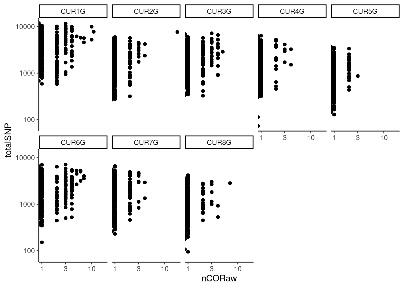
| Version | Author | Date |
|---|---|---|
| 2b964ff | rlyu | 2022-01-13 |
X-axis plots the number of haplotype transitions (nCORaw) for each cell and Y-axis plots the number of total SNPs detected in a cell. A large nCORaw might indicate the cell being a diploid cell included by accident or doublets. Cells with a lower totalSNPs might indicate poor cell quality.
A data.frame with cell-level metric is also returned:
head(pcqc$cellQC)# A tibble: 6 × 4
Chrom totalSNP nCORaw barcode
<fct> <int> <dbl> <chr>
1 CUR1G 5882 0 AAACGGGTCCAGGCGT-1
2 CUR2G 2688 1 AAACGGGTCCAGGCGT-1
3 CUR3G 2983 1 AAACGGGTCCAGGCGT-1
4 CUR4G 2851 0 AAACGGGTCCAGGCGT-1
5 CUR5G 1361 0 AAACGGGTCCAGGCGT-1
6 CUR6G 3323 1 AAACGGGTCCAGGCGT-1perSegChrQC
PerSegQC function visualizes statistics of inferred haplotype state segments, which helps decide filtering thresholds for removing crossovers that do not have enough evidence by the data and the very close double crossovers which are biologically unlikely.
psqc <- perSegChrQC("apricot",chroms=paste0("CUR",1:8,"G"),
                    path=dataset_dir,
                    barcodeFile=barcodeFile_path,
                    maxRawCO = 5)
psqc+theme_classic()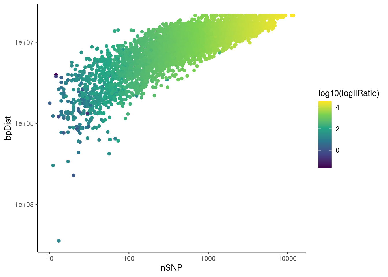
| Version | Author | Date |
|---|---|---|
| 2b964ff | rlyu | 2022-01-13 |
psqc <- perSegChrQC("apricot",chroms=paste0("CUR",8,"G"),
                    path=dataset_dir,
                    barcodeFile=barcodeFile_path,
                    maxRawCO = 10)
psqc+theme_classic()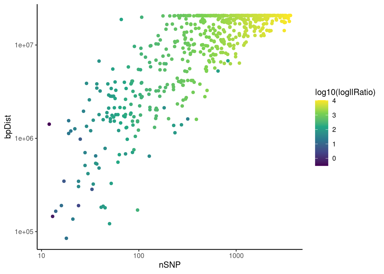
| Version | Author | Date |
|---|---|---|
| 2b964ff | rlyu | 2022-01-13 |
Parsing files using comapr
Now we have some idea about the features of this dataset, we can read in the files from sgcocaller which can be directly parsed through readHapState function. This function returns a RangedSummarizedExperiment object with rowRanges containing SNP positions that have ever contributed to crossovers in a cell, while colData contains the cell annotations such as barcodes.
The following filters have been applied:
- Segment level filters:
- minSNP=10, the segment that results in one/two crossovers has to have more than 10 SNPs of support
- minlogllRatio=5, the segment that results in one/two crossovers has to have logllRatio larger than 5
- bpDist=1e6, the segment that results in one/two crossovers has to have base pair distances larger than 1e6
- Cell level filters:
- maxRawCO, the maximum number of raw crossovers (the number of state transitions from the _vi.mtx file) for a cell
- minCellSNP=200, there have to be more than 200 SNPs detected within a cell, otherwise this cell is removed.
More description can be found from the previous analysis report.
In this set of analysis, we scaled bpDist filter by the chromosomes’ physical sizes.
chrom_size <- read.table(file = "data/chrom_size.txt", col.names = c("chrom","size"))bpDist_min <- 1e6
bpDist_min_perchrom <- bpDist_min*(chrom_size$size/chrom_size$size[1])
#bpDist_min_perchrom <- c(bpDist_min,rep(bpDist_min/10,7))
bcdf <- read.table(barcodeFile_path)
#bpDist_min_perchrom <- c(bpDist_min,rep(bpDist_min/10,7))
apricot_rse <- readHapState(sampleName = "apricot",
path = dataset_dir,
chroms =paste0("CUR",1:8,"G"),
barcodeFile = barcodeFile_path,
minSNP = 10, minCellSNP = 200,
maxRawCO = 5,
minlogllRatio = 5,
bpDist = bpDist_min_perchrom,
biasTol = 0.3 )The summary of the constructed RangedSummarizedExperiment object:
apricot_rseclass: RangedSummarizedExperiment
dim: 7206 334
metadata(10): ithSperm Seg_start ... bp_dist barcode
assays(1): vi_state
rownames: NULL
rowData names(0):
colnames(334): AAACGGGTCCAGGCGT-1 AACCGCGGTTGGTATC-1 ...
TTTATGCTCGTTAGGT-1 TTTCCTCAGCTTCAGT-1
colData names(1): barcodespublished_cos <- read.table(file = paste0(path_dir, "data/Gamete-binning-tables.txt" ),
skip = 1, header = 1)
published_cos$barcode <- sapply(stringr::str_split(published_cos$Nuclei.ID..Library_ID_barcode,"_"),`[[`,3)
published_cos$barcode <- paste0(published_cos$barcode,"-1")apricot_rse <- apricot_rse[,apricot_rse$barcodes %in% unique(published_cos$barcode)]Crossover counts
Counting the number of crossovers per gamete by countCOs:
apricot_rse_count <-  countCOs(apricot_rse)
#saveRDS(apricot_rse_count, file = "output/apricot_rse_count.knownhap.rds")
Plot the number of crossovers per gamete and per chromosome:
apricot_rse_count$sampleGroup <- "apricot"
plotCount(apricot_rse_count,group_by = "sampleGroup")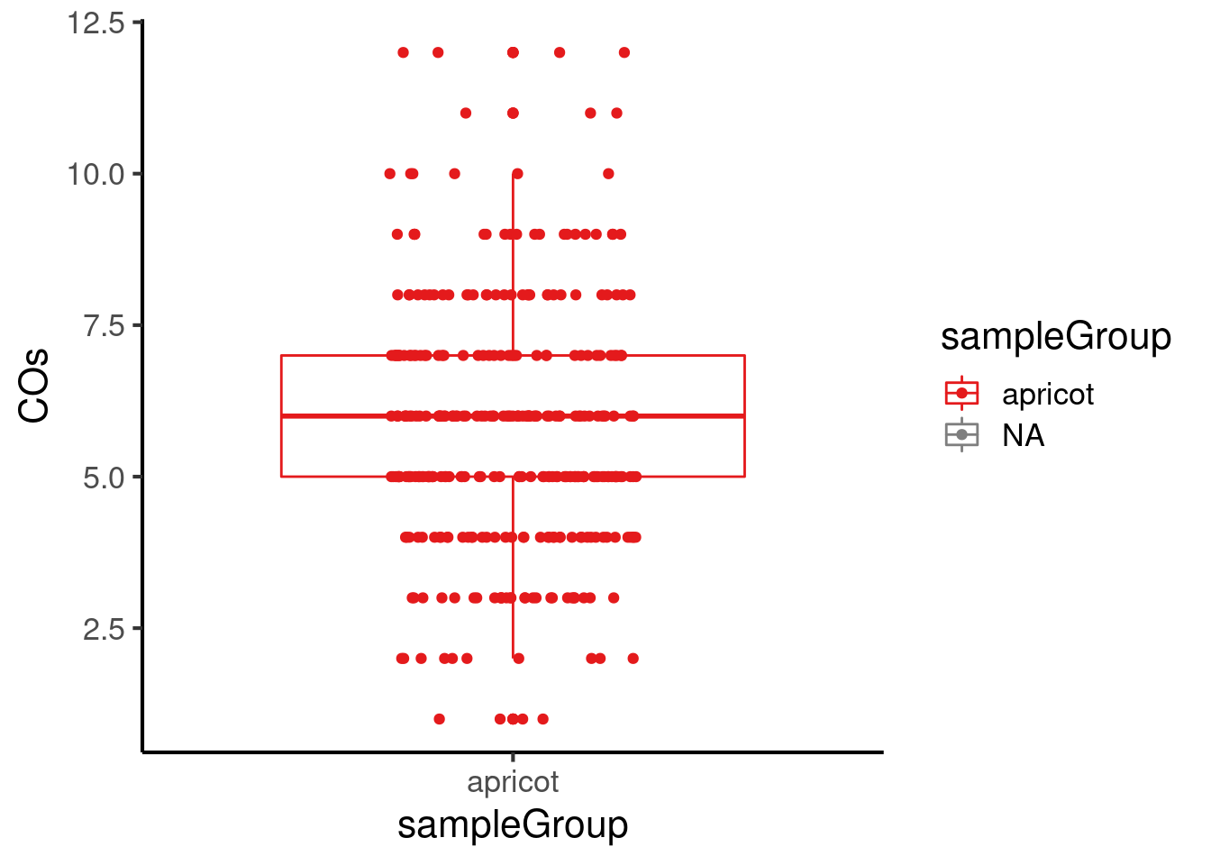
| Version | Author | Date |
|---|---|---|
| 2b964ff | rlyu | 2022-01-13 |
plotCount(apricot_rse_count,by_chr = T,plot_type = "error_bar")+theme_classic()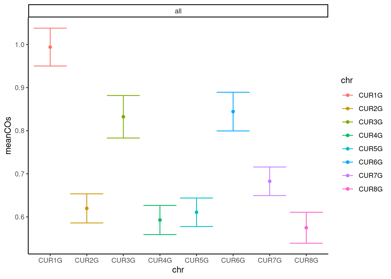
| Version | Author | Date |
|---|---|---|
| 2b964ff | rlyu | 2022-01-13 |
Compare called crossovers and published crossovers
The number of crossovers per gamete from the published study was obtained from the TableS4 (Campoy et al. 2020):
published_cos_called <- published_cos[published_cos$barcode %in% apricot_rse$barcodes,]

published_cos_df <- published_cos_called %>% dplyr::group_by(barcode,Chr) %>%
  dplyr::summarise(nCOs = n() )
`summarise()` has grouped output by 'barcode'. You can override using the `.groups` argument.#published_cos_df$Chr <- paste0("chr",stringr::str_sub(published_cos_df$Chr,4,4))
fill_chrs <- data.frame(barcode = unique(published_cos_df$barcode),
Chr = rep( paste0("CUR",1:8,"G"),
each = length(unique(published_cos_df$barcode))),
nCOs = 0)
published_cos_df <- merge(published_cos_df, fill_chrs,by =c("barcode","Chr"),all =T)
published_cos_df$nCOs <- ifelse(is.na(published_cos_df$nCOs.x),0,published_cos_df$nCOs.x)
chr_co_counts <- lapply(paste0("CUR",1:8,"G"), function(chr){
df <- colSums(as.matrix(assay(apricot_rse_count[rowRanges(apricot_rse_count)@seqnames ==chr,])))
data.frame(barcode = names(df),nCOs = round(df,2), Chr =chr)
})
called_co_df <- Reduce(rbind,chr_co_counts)
compareDf <- merge(published_cos_df,called_co_df,by = c("barcode","Chr"),
suffix = c("published","called"))Compare mean number of crossovers from the published study and sgcocaller
(meanpublished <- compareDf %>% dplyr::group_by(barcode) %>%
   summarise(publishedCellCOs = sum(nCOspublished)) %>% summarise(mean(publishedCellCOs)))
# A tibble: 1 × 1
`mean(publishedCellCOs)`
<dbl>
1 5.93(meansgcocaller <- compareDf %>% dplyr::group_by(barcode) %>%
summarise(sgcocallerCellCOs = sum( nCOscalled)) %>% summarise(mean(sgcocallerCellCOs)))# A tibble: 1 × 1
`mean(sgcocallerCellCOs)`
<dbl>
1 5.75compareDf %>% dplyr::group_by(barcode) %>%
summarise(publishedCellCOs = sum( nCOspublished),
sgcocallerCellCOs = sum( nCOscalled)) %>%
tidyr::pivot_longer(cols = c("publishedCellCOs","sgcocallerCellCOs"),
names_to = "group",
values_to = "crossovers") %>%
ggplot(aes(x = group, y = crossovers))+geom_boxplot()+
geom_jitter()+theme_classic(base_size = 18)+
geom_label(aes(x=c("publishedCellCOs"),
y = 16,
label = round(meanpublished,2)),
size = 8)+
geom_label(aes(x=c("sgcocallerCellCOs"),
y = 16,
label = round(meansgcocaller,2)), size = 8)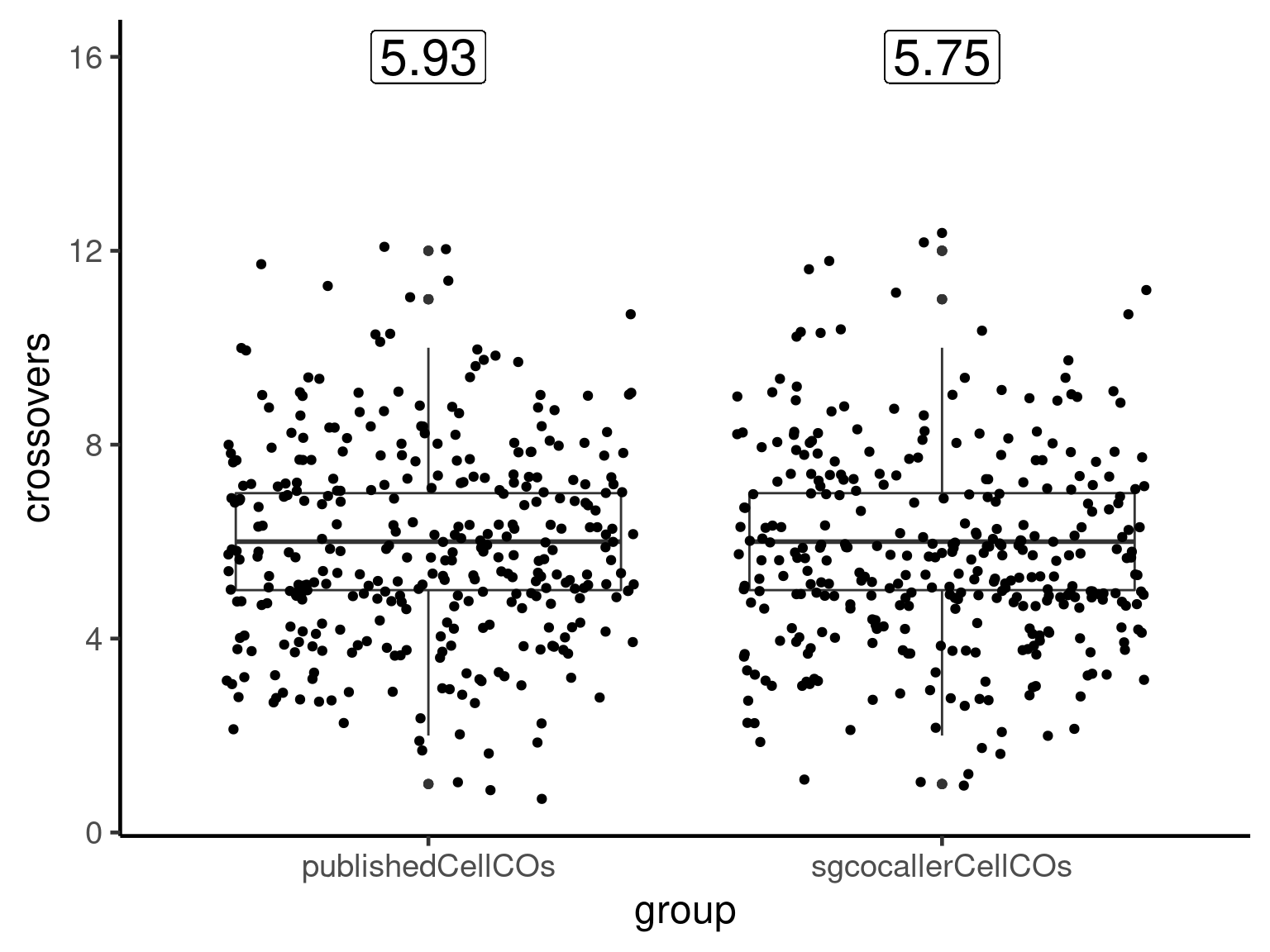
Compare total crossovers per barcode
compareDf %>% dplyr::group_by(barcode) %>%
  summarise(publishedCellCOs = sum( nCOspublished),
            sgcocallerCellCOs = sum( nCOscalled)) %>%
  ggplot(mapping = aes(x = sgcocallerCellCOs, y = publishedCellCOs)) +
  geom_point()+
  geom_jitter(mapping = aes(color = as.factor(abs(publishedCellCOs -sgcocallerCellCOs ))),
              height = 0.01)+
  scale_color_viridis_d()+theme_classic(base_size = 18)+theme(
  legend.position = c(0.15, 0.8), # c(0,0) bottom left, c(1,1) top-right.
)+guides(color=guide_legend(title="difference"))+
  xlab("COs_sgcocaller")+
  ylab("COs_campoy")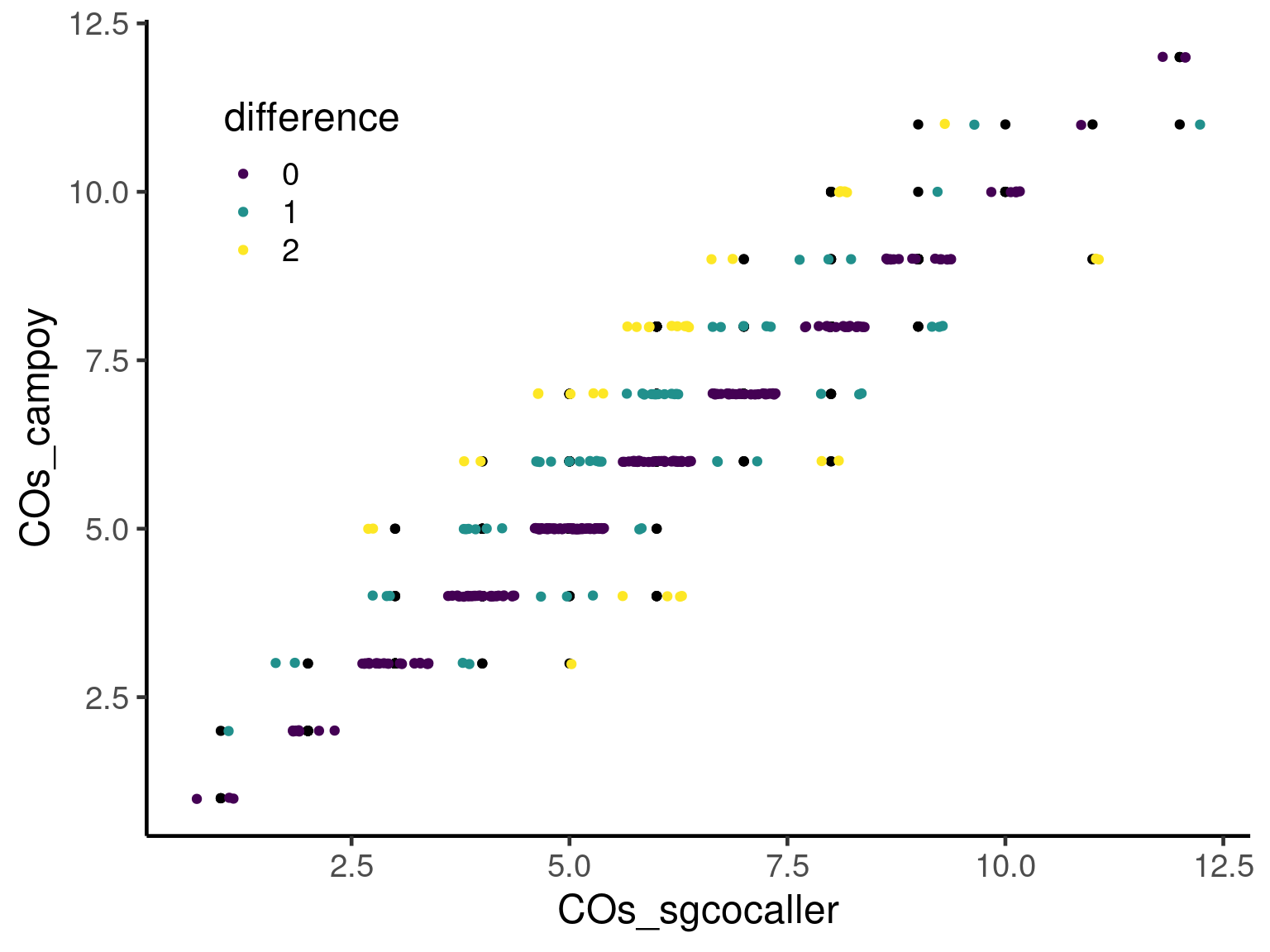
| Version | Author | Date |
|---|---|---|
| 2b964ff | rlyu | 2022-01-13 |
Differences in crossovers per chromosome from the published crossover results
compareDf$diff <- compareDf$nCOscalled-compareDf$nCOspublishedcompareDf %>% mutate(diff=as.factor(abs(diff))) %>% ggplot()+
geom_bar(mapping = aes(x = "difference",fill=diff),width=0.1,position = "fill")+
theme_classic(base_size = 18)+scale_fill_viridis_d()+facet_wrap(.~Chr)+
theme( legend.position = c(0.82, 0.15))+guides(fill=guide_legend(title="difference"))+
ylab("frequency")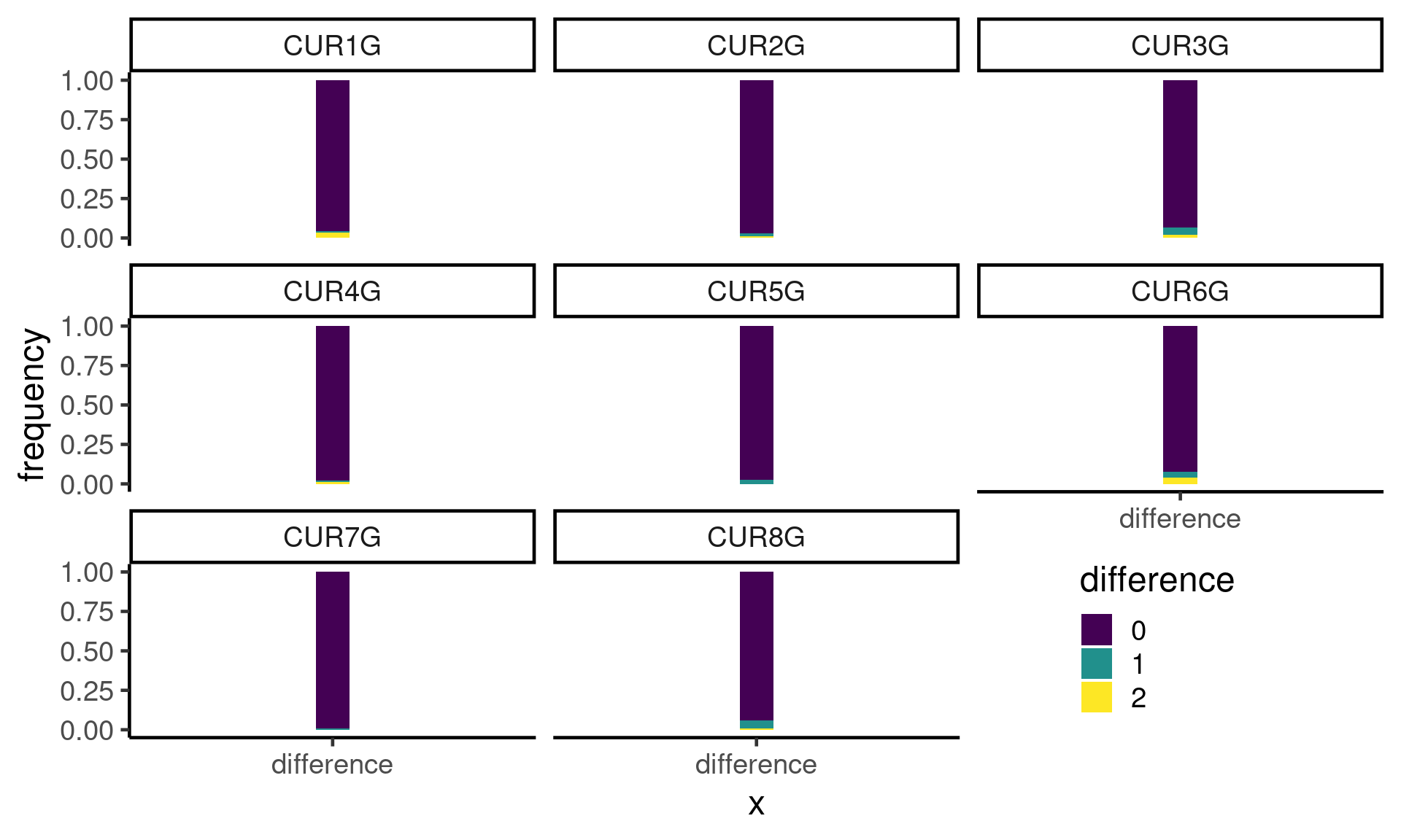
Plot alternative allele frequencies with crossover region highlighted
We choose a cell and plot the AF (alternative allele frequency) track with called crossover region highlighted.
options(ucscChromosomeNames=FALSE)
chr <- "CUR1G"
cellbc <- colnames(apricot_rse_count)[3]
cell_af <- getCellAFTrack(chrom = chr,
               path_loc = dataset_dir,
               sampleName = "apricot",
               barcodeFile = barcodeFile_path,
               nwindow = 350,
               cellBarcode = cellbc,
               co_count = apricot_rse_count)
Generate a Highlight track with the returned list object cell_af
ht <- HighlightTrack(cell_af$af_track,
                     range = cell_af$co_range[seqnames(cell_af$co_range)==chr],
                     chromosome = chr)

plotTracks(ht)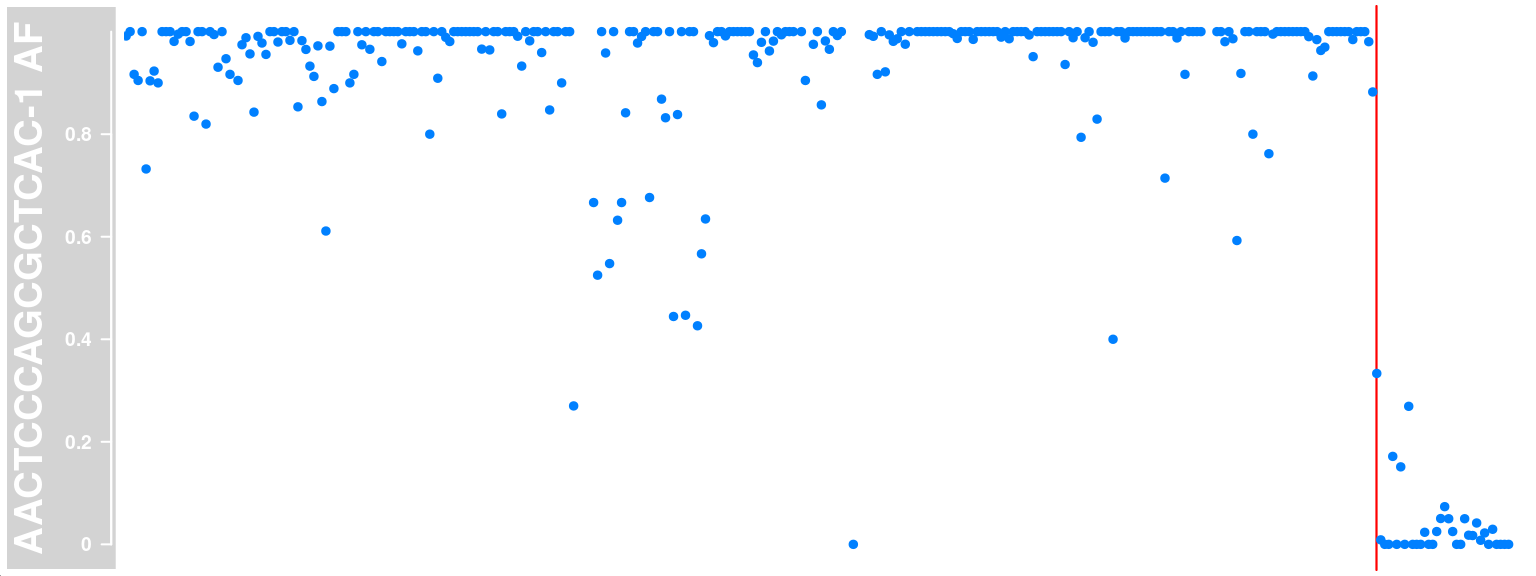
| Version | Author | Date |
|---|---|---|
| 2b964ff | rlyu | 2022-01-13 |
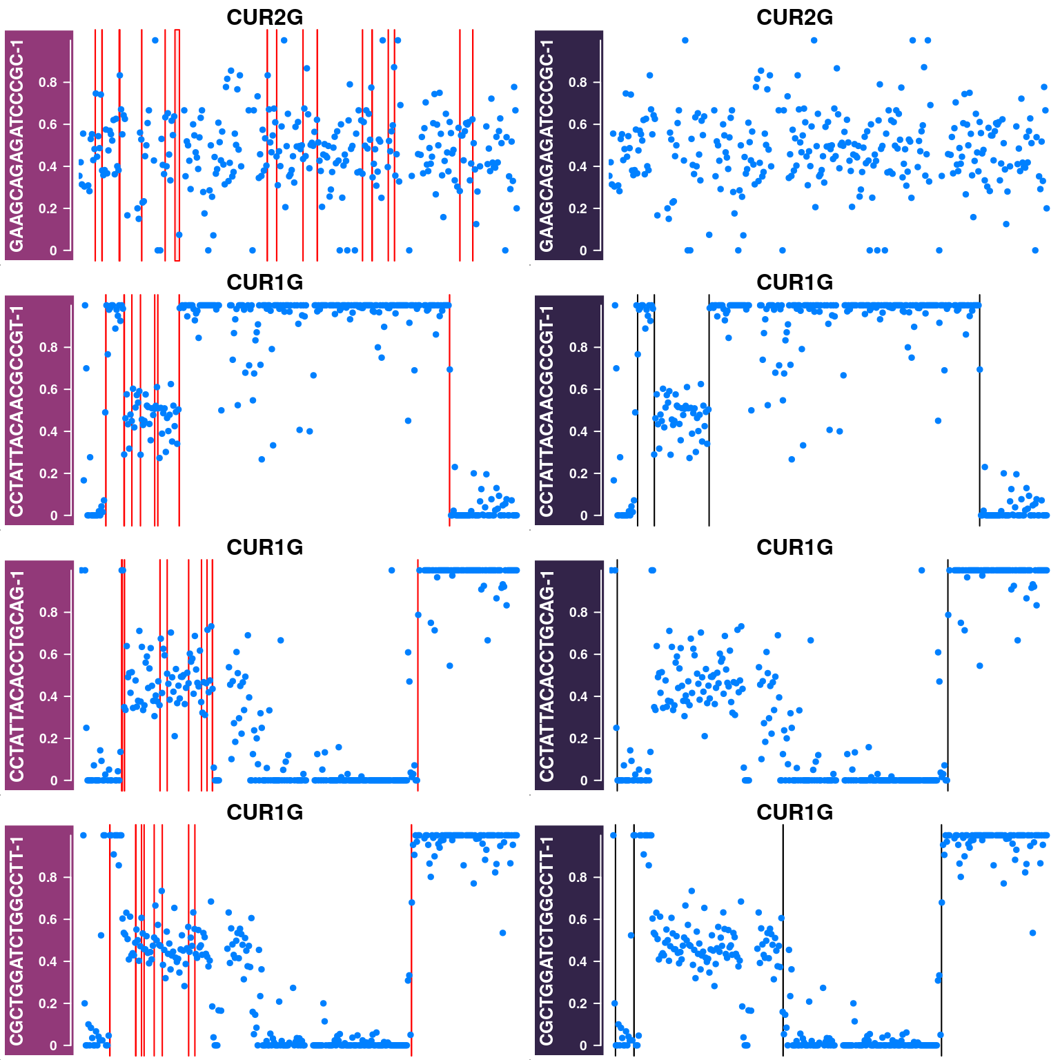
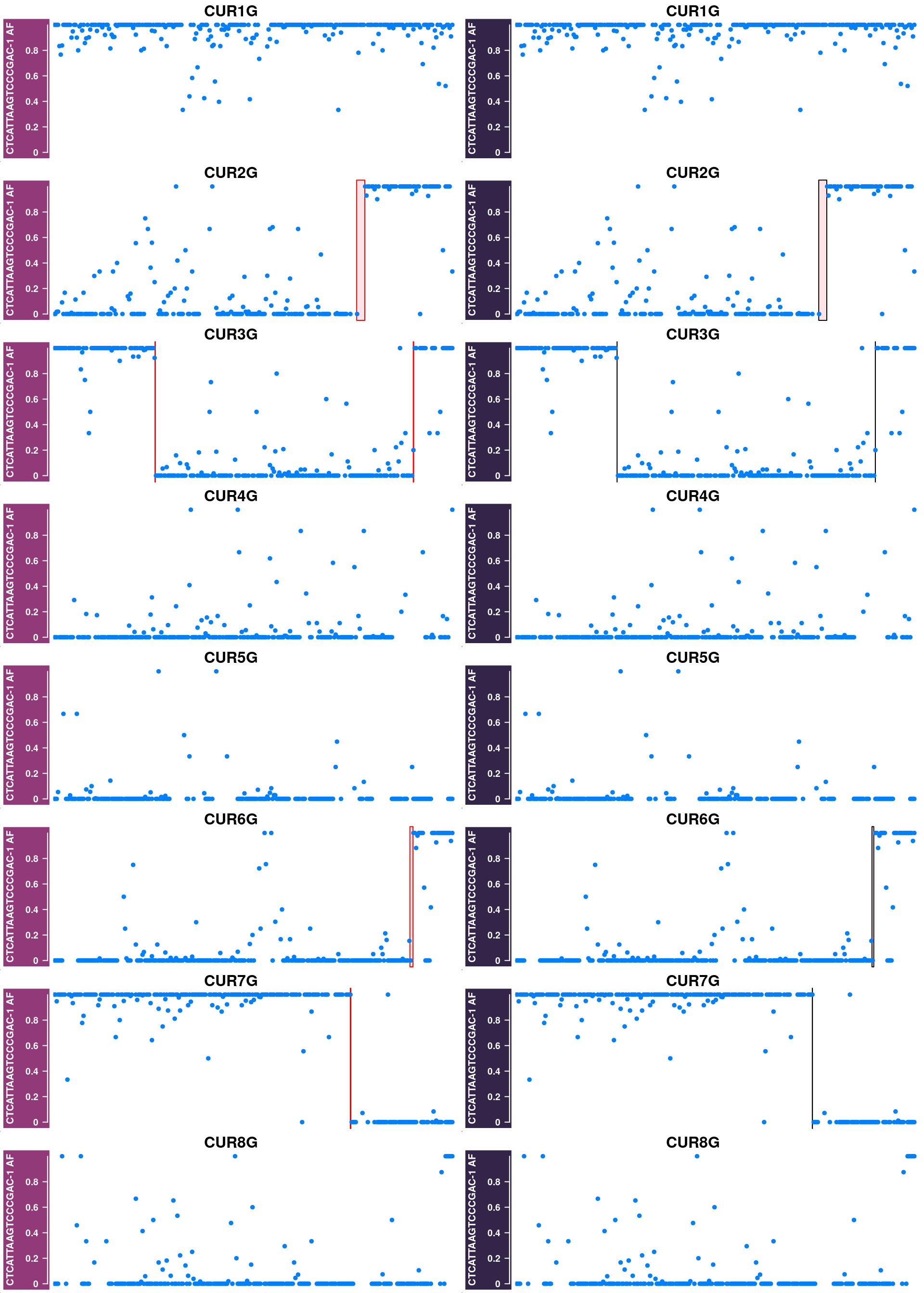
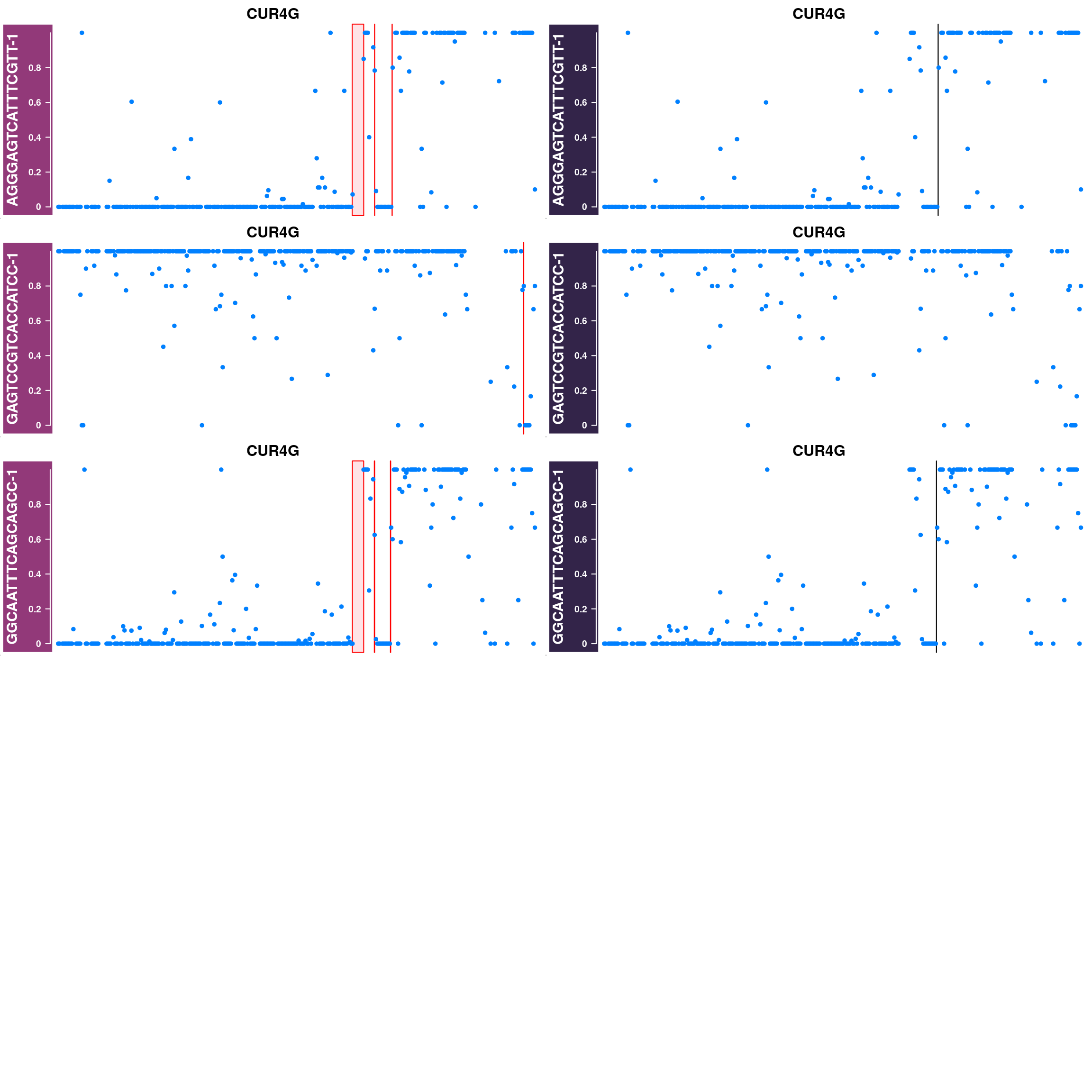
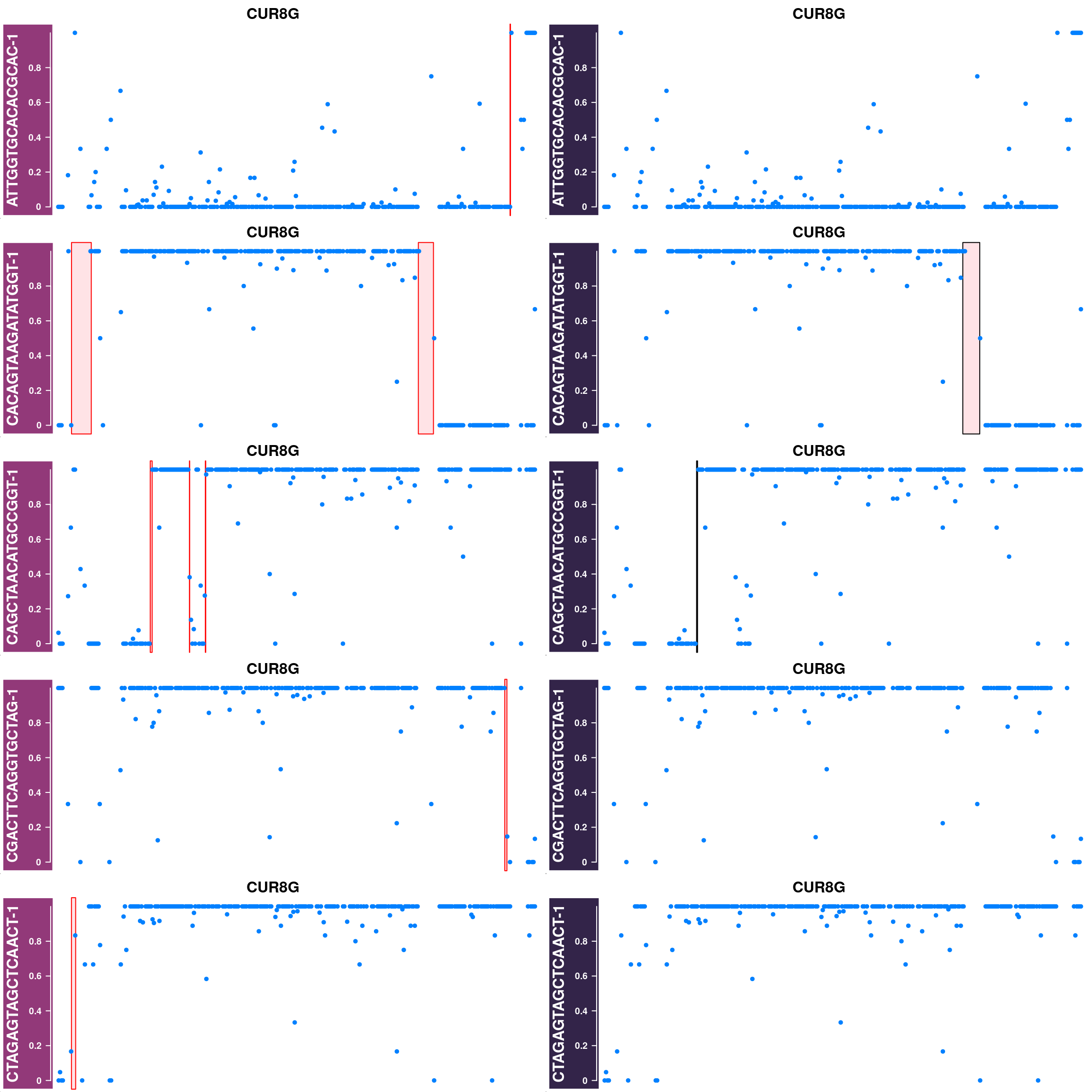
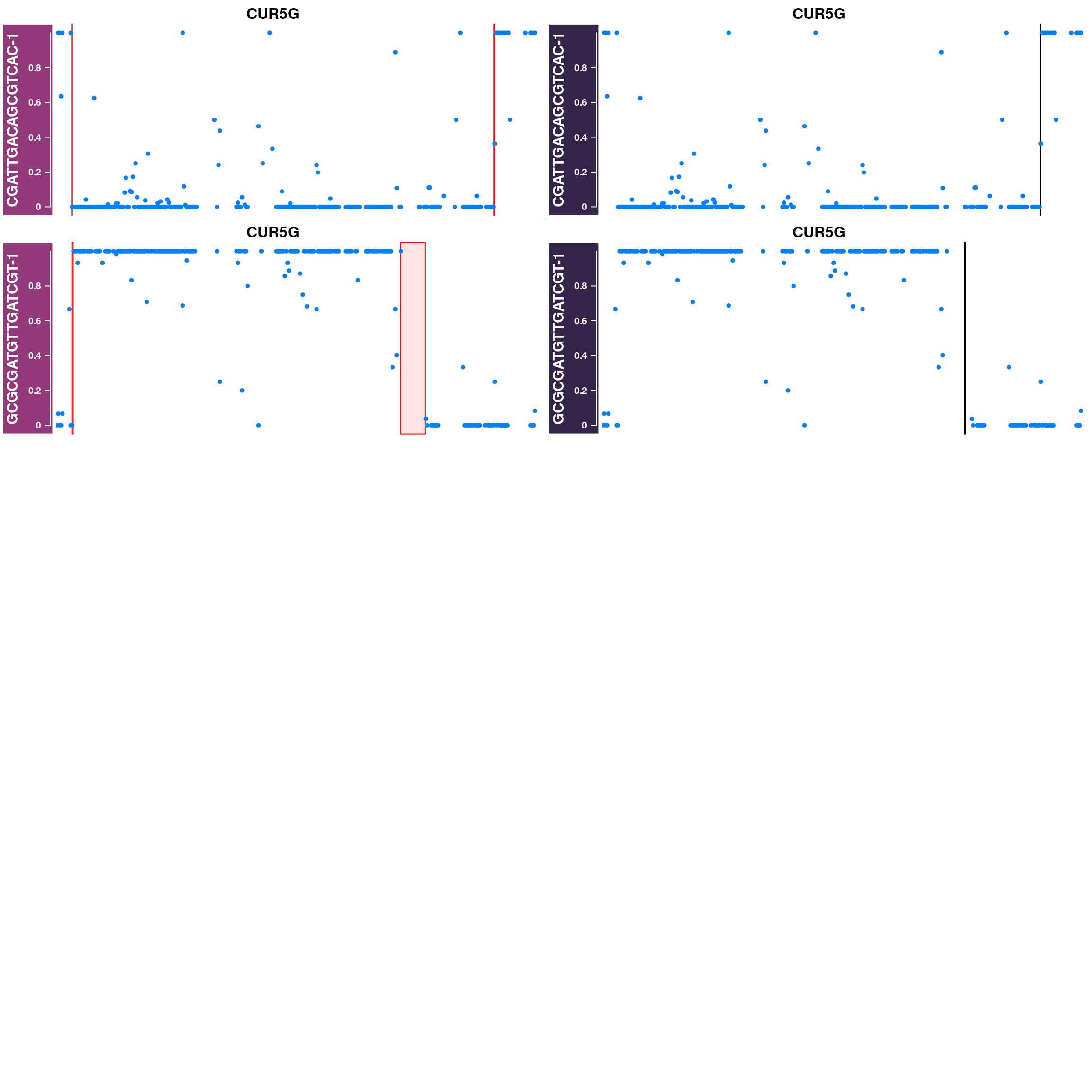
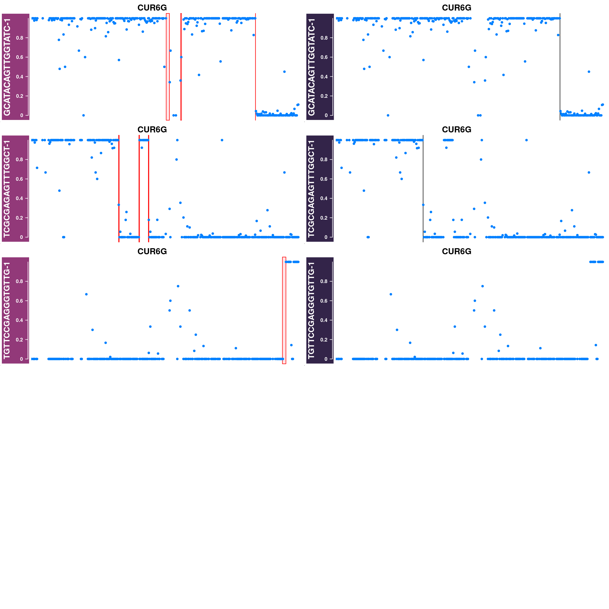
Plot cells that were removed in the first step
The cells were filtered out are cells with poor SNP coverage or cells that have been called with excessive number of crossovers due to doublet or with abnormal chromosomes as haploid cells.
plotWhoeGenomeAFtracks <- function( nrows = 10,
                                    ncols = 2,
                                    chroms = paste0("CUR",rep(1:8,each=2),"G"),
                                    ht_tracklist){
  grid.newpage()
  pushViewport(viewport(layout = grid.layout(nrows,ncols)))

  for (i in seq_along(ht_tracklist)) {
    pushViewport(viewport(layout.pos.col = ((i - 1)%%ncols) + 1,
                          layout.pos.row = (((i) - 1)%/%ncols) + 1))
    plotTracks(ht_tracklist[i],
               chromosome = chroms[i], add = TRUE,main=paste0(chroms[i]),
               cex.main = 1)
    popViewport(1)
  }
}
Get the called crossovers from published results:
apricot_rse_count_allcell <-readHapState(sampleName = "apricot",
                            path = dataset_dir,
                            chroms =paste0("CUR",1:8,"G"),
                            barcodeFile = barcodeFile_path,
                            minSNP = 0, minCellSNP = 200,
                            maxRawCO = 50,
                            minlogllRatio = 5,
                            bpDist = 0,
                            biasTol = 0.3 )
apricot_rse_count_allcell <- countCOs(apricot_rse_count_allcell)
published_cos <- read.table(file = paste0(path_dir, "data/Gamete-binning-tables.txt" ),
skip = 1, header = 1)
published_cos$barcode <- sapply(stringr::str_split(published_cos$Nuclei.ID..Library_ID_barcode,"_"),`[[`,3)
published_cos$barcode <- paste0(published_cos$barcode,"-1")
knownCO_range <- GRanges(seqnames =published_cos$Chr,
ranges = IRanges(start = published_cos$CO.Interval.Start,
end = published_cos$CO.Interval.End),
barcode = published_cos$barcode)Doublet-like cells or cells with abnormal chromosomes:
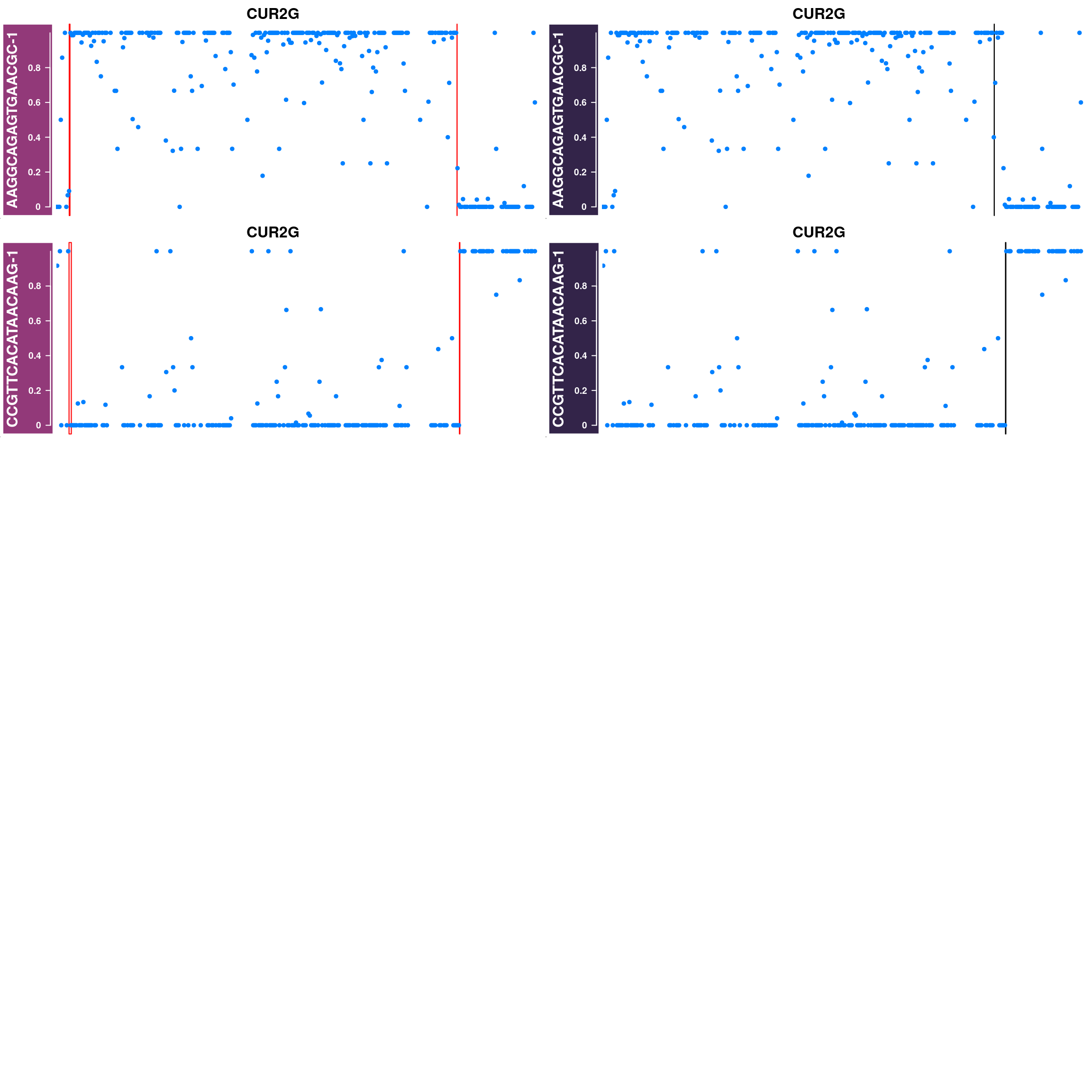
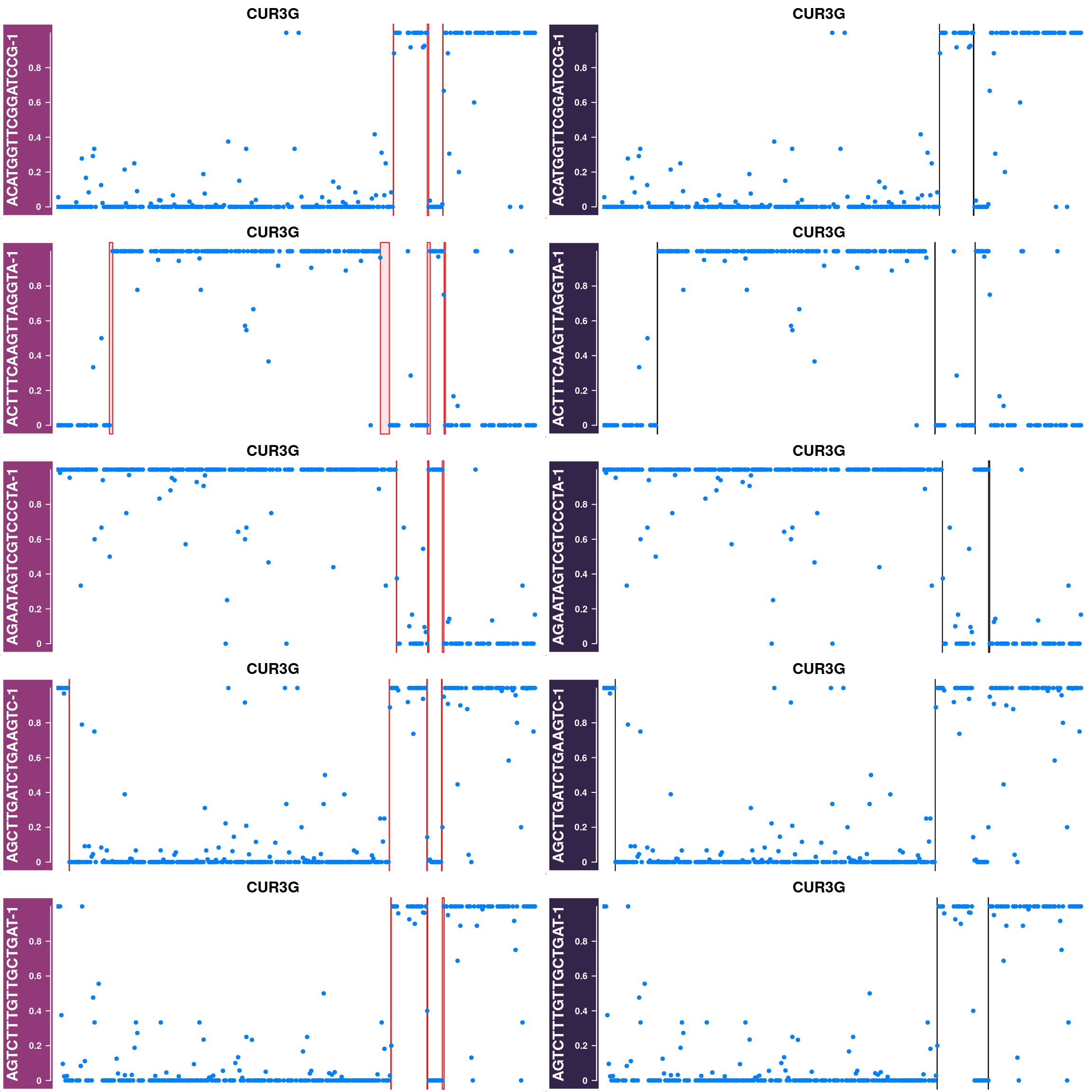
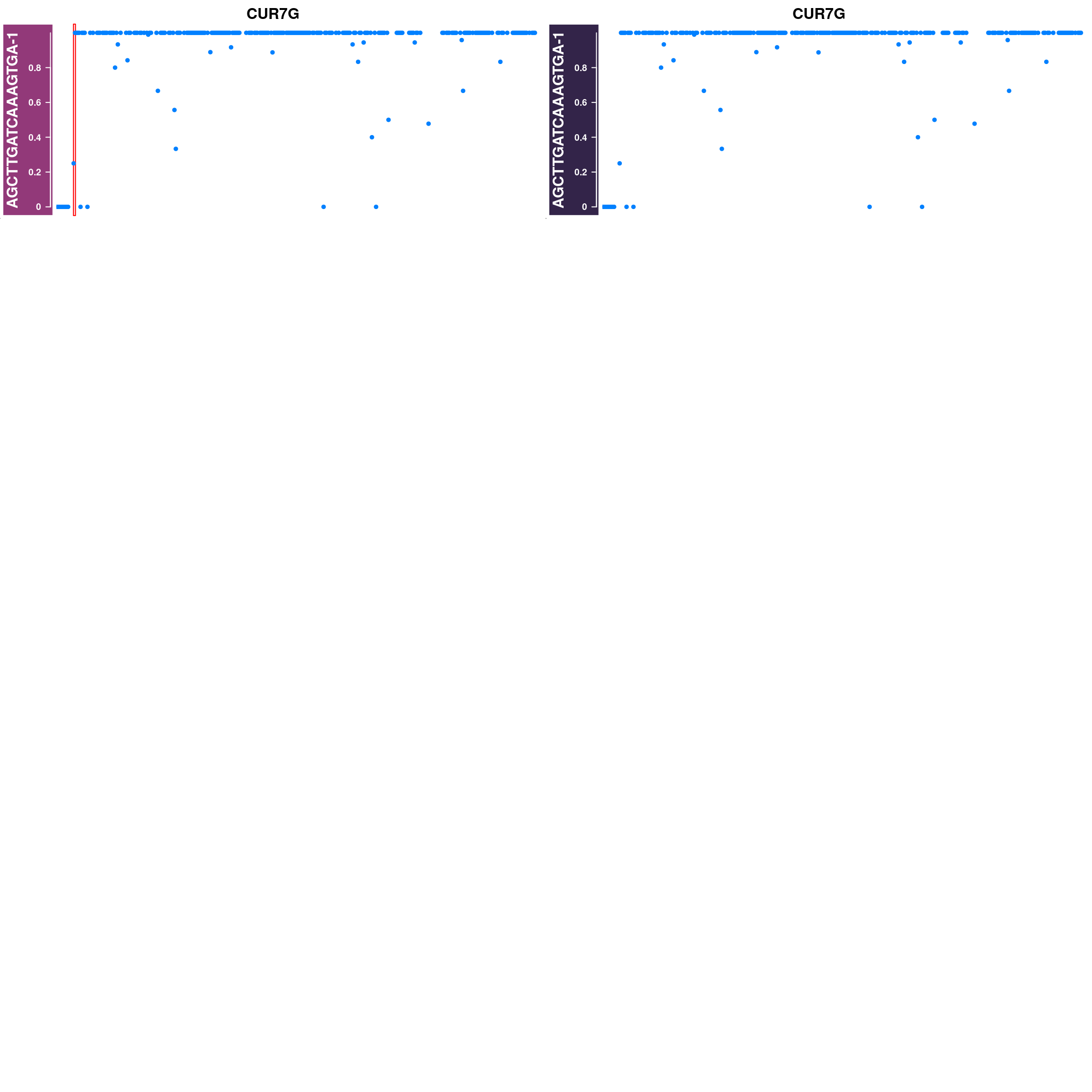
Left column plots the AF tracks for each chromosome in each cell and with called crossover regions from sgcocaller highlighted.
Right column plots the AF tracks for each chromosome in each cell and with called crossover regions from published study highlighted.
excessiveCO_chrs <- pcqc$cellQC %>% filter(pcqc$cellQC$nCORaw>8)
exceChrBC_ht_list <- list()
for(i in seq(nrow(excessiveCO_chrs))){

  cellbc <- as.character(excessiveCO_chrs$barcode)[i]
  chr <- as.character(excessiveCO_chrs$Chrom)[i]
  af_track<- comapr::getCellAFTrack(chrom = chr,
                                      nwindow = 350,
                                      path_loc = dataset_dir,
                                      sampleName = "apricot",
                                      barcodeFile = barcodeFile_path,
                                      cellBarcode = cellbc,
                                      co_count = apricot_rse_count_allcell)

  suppressMessages(names(af_track$af_track) <- paste0(cellbc))

  suppressMessages(aftrack1 <- setPar(af_track$af_track, name="background.title",
                                        value = "#923979"))
  ht1 <- HighlightTrack(aftrack1,
                       range = af_track$co_range[seqnames(af_track$co_range)==chr],
                       chromosome = chr)
  knownCO_range_bc <- knownCO_range[knownCO_range$barcode == cellbc,]
  suppressMessages(aftrack2 <- setPar(af_track$af_track, name="background.title",
                                      value = "#332449"))
  if(length(knownCO_range_bc) == 0){
      ht2 <-aftrack2
  } else {
      ht2 <- HighlightTrack(aftrack2,
                        range = knownCO_range_bc[seqnames(knownCO_range_bc)==chr],
                        col = "black",
                        chromosome = chr,
                        names = "published")
  }

  exceChrBC_ht_list <- c(exceChrBC_ht_list, ht1,ht2)
}


saveRDS(exceChrBC_ht_list,file = "output/exceChrBC_ht_list.rds")
excessiveCO_chrs <- pcqc$cellQC %>% filter(pcqc$cellQC$nCORaw>8)
exceChrBC_ht_list <- readRDS("output/exceChrBC_ht_list.rds")
nrows = 4
ncols = 2
grid.newpage()
pushViewport(viewport(layout = grid.layout(nrows,ncols)))
chroms <- rep( as.character(excessiveCO_chrs$Chrom),each=2)
# seq(exceChrBC_ht_list)
for(i in c(1:8) ){
chr <- chroms[i]
k <- ifelse(i%%(nrows*ncols)>0,i%%(nrows*ncols),8)
# message(k)
pushViewport(viewport(layout.pos.col = ((k - 1)%%ncols) + 1,
layout.pos.row = (((k) - 1)%/%ncols) + 1))
plotTracks(exceChrBC_ht_list[i],
chromosome =chr, add = TRUE,
main=paste0(chr),
cex.main = 1)
popViewport(1)
}
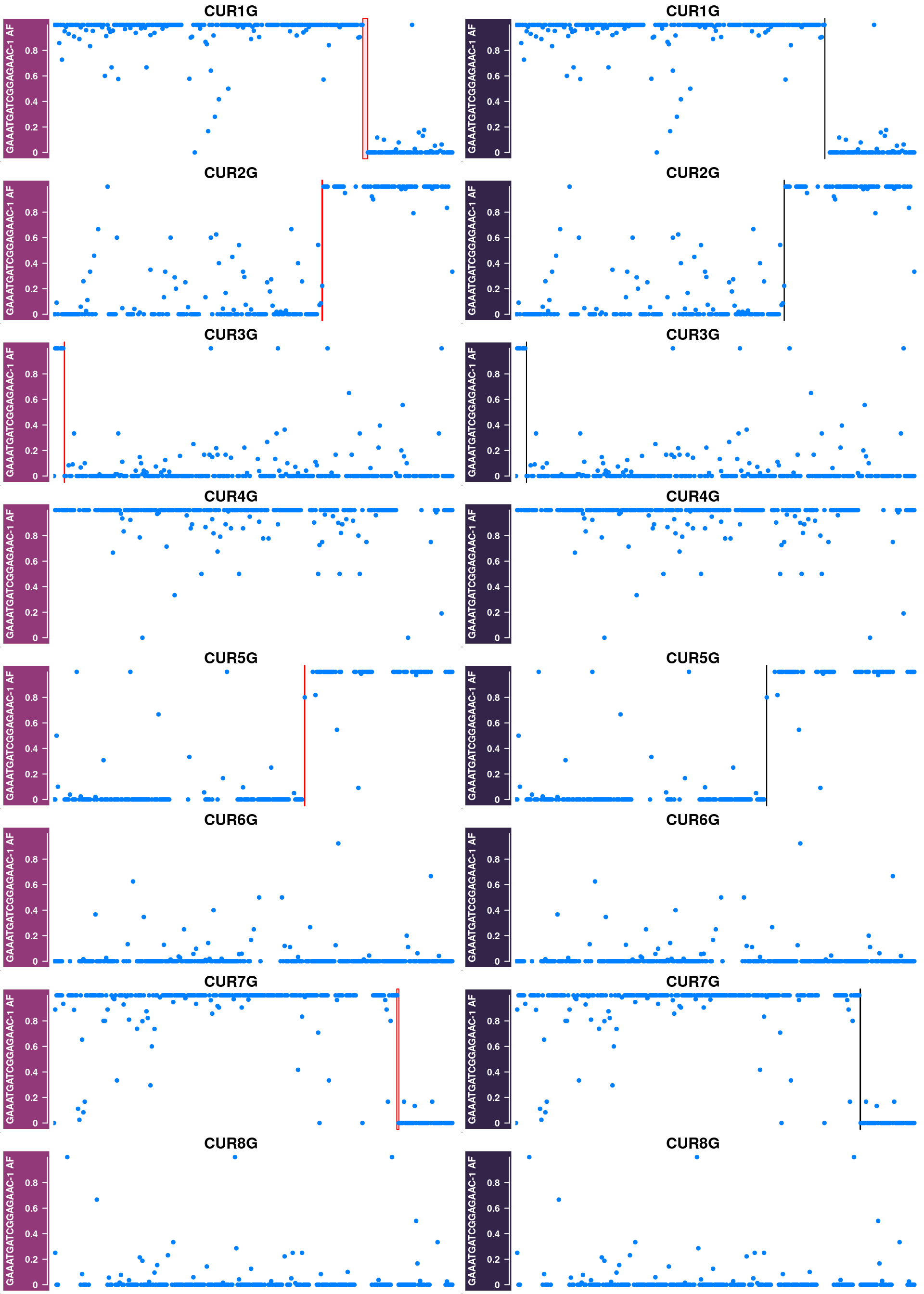
Generate supplimentary figure showing randomly selected AF tracks with CO interval
highlighted
Cell AF (alternative allele frequency) tracks with CO interval highlighted
for(cellbc in apricot_rse_count$barcodes[sample(ncol(apricot_rse_count),3)]) {
  htlist <- list()
  for(chr in paste0("CUR",seq(8),"G")){

    af_track<- getCellAFTrack(chrom = chr, nwindow = 300,
                              path_loc = dataset_dir,
                              sampleName = "apricot",
                              barcodeFile = barcodeFile_path,
                              cellBarcode = cellbc,
                              co_count = apricot_rse_count,
                              chunk = 10000)

    suppressMessages(af_track$af_track <- Gviz::setPar(af_track$af_track,"name",
                                                       paste0(cellbc,chr)))
    suppressMessages(aftrack1 <- setPar(af_track$af_track, name="background.title",
                                        value = "#923979"))
    ht1 <- HighlightTrack(aftrack1,
                         range = af_track$co_range[seqnames(af_track$co_range)==chr],
                         chromosome = chr)


    knownCO_range_bc <- knownCO_range[knownCO_range$barcode == cellbc,]
    suppressMessages(aftrack2 <- setPar(af_track$af_track, name="background.title",
                                        value = "#332449"))
    ht2 <- HighlightTrack(aftrack2,
                          range = knownCO_range_bc[seqnames(knownCO_range_bc)==chr],
                          col = "black",
                          chromosome = chr)

    htlist <- c(htlist, ht1,ht2)
  }

  plotWhoeGenomeAFtracks(nrows = 8,ncols = 2,
                       ht_tracklist = htlist)
}
| Version | Author | Date |
|---|---|---|
| 69a77e3 | rlyu | 2021-07-19 |
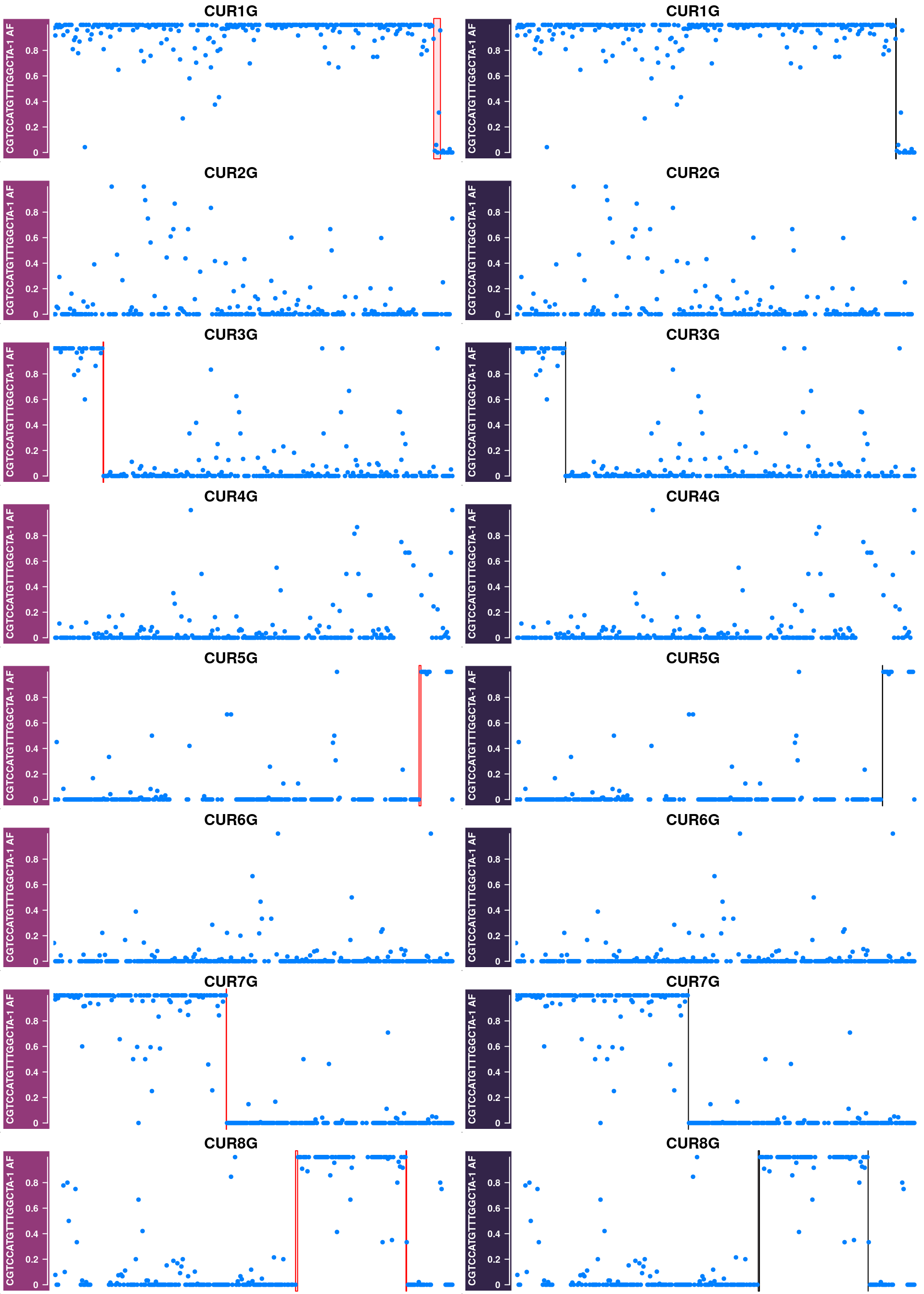
Some example chromosomes with discrepancy in called crossovers from sgcocaller and the published crossovers:
## plot 20 for each chrom
disChrBC <- compareDf %>% filter(diff>0)
#pdf(paste0("output/discrepancyChrsR3A7_1e6scaled.pdf"),height = 16,width = 12,pointsize = 8)

for(chr in unique(disChrBC$Chr)){
  disChrBC_ht_list <- list()

  for(i in which(disChrBC$Chr==chr)){
    #chr <- disChrBC[i,"Chr"]
    cellbc <- disChrBC[i,"barcode"]

    af_track<- comapr::getCellAFTrack(chrom = chr,
                                      nwindow = 350,
                                      path_loc = dataset_dir,
                                      sampleName = "apricot",
                                      barcodeFile = barcodeFile_path,
                                      cellBarcode = cellbc,
                                      co_count = apricot_rse_count)

    suppressMessages(names(af_track$af_track) <- paste0(cellbc))
                       #Gviz::setPar(af_track$af_track,"name",
                      #                                   paste0(cellbc,chr)))
    suppressMessages(aftrack1 <- setPar(af_track$af_track, name="background.title",
                                        value = "#923979"))
    ht1 <- HighlightTrack(aftrack1,
                         range = af_track$co_range[seqnames(af_track$co_range)==chr],
                         chromosome = chr)


    knownCO_range_bc <- knownCO_range[knownCO_range$barcode == cellbc,]
    suppressMessages(aftrack2 <- setPar(af_track$af_track, name="background.title",
                                        value = "#332449"))

    ht2 <- HighlightTrack(aftrack2,
                          range = knownCO_range_bc[seqnames(knownCO_range_bc)==chr],
                          col = "black",
                          chromosome = chr,
                          names = "published")
    disChrBC_ht_list <- c(disChrBC_ht_list, ht1,ht2)
    if(length(disChrBC_ht_list)>9){
      break
    }
  }

  nrows = 5
  ncols = 2
  chroms <- rep( rep(chr,5),each=2)
  for(i in seq(disChrBC_ht_list) ){
    if(i%%(nrows*ncols)==1){
      grid.newpage()
      pushViewport(viewport(layout = grid.layout(nrows,ncols)))
    }
    chr <-  disChrBC[i,"Chr"]
    k <- ifelse(i%%(nrows*ncols)>0,i%%(nrows*ncols),10)
    pushViewport(viewport(layout.pos.col = ((k - 1)%%ncols) + 1,
                          layout.pos.row = (((k) - 1)%/%ncols) + 1))

    plotTracks(disChrBC_ht_list[i],
               chromosome =chroms[i], add = TRUE,
               main=paste0(chroms[i]),
                 cex.main = 1)
    popViewport(1)

  }

}
| Version | Author | Date |
|---|---|---|
| 306d81f | rlyu | 2021-07-20 |
Conclusion
Using sgcocaller and comapr has returned a highly concordant crossover profiles for the group of gametes analyzed with the published study. In addition, it skipped the step of splitting the Bam file to individual single-gamete bam files for crossover identification which saves much time and computational resources. It is able to generate covenient summary plots and visulisation of crossover events nicely.
Sessioninfo
sessionInfo()R version 4.1.0 (2021-05-18)
Platform: x86_64-pc-linux-gnu (64-bit)
Running under: Rocky Linux 8.5 (Green Obsidian)
Matrix products: default
BLAS/LAPACK: /usr/lib64/libopenblasp-r0.3.12.so
locale:
[1] LC_CTYPE=en_AU.UTF-8 LC_NUMERIC=C
[3] LC_TIME=en_AU.UTF-8 LC_COLLATE=en_AU.UTF-8
[5] LC_MONETARY=en_AU.UTF-8 LC_MESSAGES=en_AU.UTF-8
[7] LC_PAPER=en_AU.UTF-8 LC_NAME=C
[9] LC_ADDRESS=C LC_TELEPHONE=C
[11] LC_MEASUREMENT=en_AU.UTF-8 LC_IDENTIFICATION=C
attached base packages:
[1] grid parallel stats4 stats graphics grDevices utils
[8] datasets methods base
other attached packages:
[1] Matrix_1.3-3 SummarizedExperiment_1.22.0
[3] Biobase_2.52.0 MatrixGenerics_1.4.3
[5] matrixStats_0.61.0 Gviz_1.36.2
[7] GenomicRanges_1.44.0 GenomeInfoDb_1.28.4
[9] IRanges_2.26.0 S4Vectors_0.30.1
[11] BiocGenerics_0.38.0 dplyr_1.0.7
[13] ggplot2_3.3.5 comapr_0.99.37
loaded via a namespace (and not attached):
[1] backports_1.2.1 circlize_0.4.13 Hmisc_4.5-0
[4] workflowr_1.6.2 BiocFileCache_2.0.0 plyr_1.8.6
[7] lazyeval_0.2.2 splines_4.1.0 BiocParallel_1.26.2
[10] digest_0.6.28 foreach_1.5.1 ensembldb_2.16.4
[13] htmltools_0.5.2 fansi_0.5.0 magrittr_2.0.1
[16] checkmate_2.0.0 memoise_2.0.0 BSgenome_1.60.0
[19] cluster_2.1.2 Biostrings_2.60.2 prettyunits_1.1.1
[22] jpeg_0.1-9 colorspace_2.0-2 blob_1.2.2
[25] rappdirs_0.3.3 xfun_0.26 crayon_1.4.1
[28] RCurl_1.98-1.5 jsonlite_1.7.2 survival_3.2-11
[31] VariantAnnotation_1.38.0 iterators_1.0.13 glue_1.4.2
[34] gtable_0.3.0 zlibbioc_1.38.0 XVector_0.32.0
[37] DelayedArray_0.18.0 shape_1.4.6 scales_1.1.1
[40] DBI_1.1.1 Rcpp_1.0.7 viridisLite_0.4.0
[43] progress_1.2.2 htmlTable_2.2.1 foreign_0.8-81
[46] bit_4.0.4 Formula_1.2-4 htmlwidgets_1.5.4
[49] httr_1.4.2 RColorBrewer_1.1-2 ellipsis_0.3.2
[52] pkgconfig_2.0.3 XML_3.99-0.8 farver_2.1.0
[55] nnet_7.3-16 dbplyr_2.1.1 utf8_1.2.2
[58] labeling_0.4.2 tidyselect_1.1.1 rlang_0.4.11
[61] reshape2_1.4.4 later_1.3.0 AnnotationDbi_1.54.1
[64] munsell_0.5.0 tools_4.1.0 cachem_1.0.6
[67] cli_3.0.1 generics_0.1.0 RSQLite_2.2.8
[70] evaluate_0.14 stringr_1.4.0 fastmap_1.1.0
[73] yaml_2.2.1 knitr_1.36 bit64_4.0.5
[76] fs_1.5.0 purrr_0.3.4 KEGGREST_1.32.0
[79] AnnotationFilter_1.16.0 whisker_0.4 xml2_1.3.2
[82] biomaRt_2.48.3 compiler_4.1.0 rstudioapi_0.13
[85] plotly_4.9.4.1 filelock_1.0.2 curl_4.3.2
[88] png_0.1-7 tibble_3.1.4 stringi_1.7.4
[91] highr_0.9 GenomicFeatures_1.44.2 lattice_0.20-44
[94] ProtGenerics_1.24.0 vctrs_0.3.8 pillar_1.6.3
[97] lifecycle_1.0.1 jquerylib_0.1.4 GlobalOptions_0.1.2
[100] data.table_1.14.2 bitops_1.0-7 httpuv_1.6.3
[103] rtracklayer_1.52.1 R6_2.5.1 BiocIO_1.2.0
[106] latticeExtra_0.6-29 promises_1.2.0.1 gridExtra_2.3
[109] codetools_0.2-18 dichromat_2.0-0 assertthat_0.2.1
[112] rprojroot_2.0.2 rjson_0.2.20 withr_2.4.2
[115] GenomicAlignments_1.28.0 Rsamtools_2.8.0 GenomeInfoDbData_1.2.6
[118] hms_1.1.1 rpart_4.1-15 tidyr_1.1.4
[121] rmarkdown_2.11 git2r_0.28.0 biovizBase_1.40.0
[124] base64enc_0.1-3 restfulr_0.0.13
devtools::session_info()─ Session info ───────────────────────────────────────────────────────────────
setting value
version R version 4.1.0 (2021-05-18)
os Rocky Linux 8.5 (Green Obsidian)
system x86_64, linux-gnu
ui X11
language (EN)
collate en_AU.UTF-8
ctype en_AU.UTF-8
tz Australia/Melbourne
date 2022-01-20
─ Packages ───────────────────────────────────────────────────────────────────
package * version date lib source
AnnotationDbi 1.54.1 2021-06-08 [1] Bioconductor
AnnotationFilter 1.16.0 2021-05-19 [1] Bioconductor
assertthat 0.2.1 2019-03-21 [1] CRAN (R 4.1.0)
backports 1.2.1 2020-12-09 [1] CRAN (R 4.1.0)
base64enc 0.1-3 2015-07-28 [1] CRAN (R 4.1.0)
Biobase * 2.52.0 2021-05-19 [1] Bioconductor
BiocFileCache 2.0.0 2021-05-19 [1] Bioconductor
BiocGenerics * 0.38.0 2021-05-19 [1] Bioconductor
BiocIO 1.2.0 2021-05-19 [1] Bioconductor
BiocParallel 1.26.2 2021-08-22 [1] Bioconductor
biomaRt 2.48.3 2021-08-15 [1] Bioconductor
Biostrings 2.60.2 2021-08-05 [1] Bioconductor
biovizBase 1.40.0 2021-05-19 [1] Bioconductor
bit 4.0.4 2020-08-04 [1] CRAN (R 4.1.0)
bit64 4.0.5 2020-08-30 [1] CRAN (R 4.1.0)
bitops 1.0-7 2021-04-24 [1] CRAN (R 4.1.0)
blob 1.2.2 2021-07-23 [1] CRAN (R 4.1.0)
BSgenome 1.60.0 2021-05-19 [1] Bioconductor
cachem 1.0.6 2021-08-19 [1] CRAN (R 4.1.0)
callr 3.7.0 2021-04-20 [1] CRAN (R 4.1.0)
checkmate 2.0.0 2020-02-06 [1] CRAN (R 4.1.0)
circlize 0.4.13 2021-06-09 [1] CRAN (R 4.1.0)
cli 3.0.1 2021-07-17 [1] CRAN (R 4.1.0)
cluster 2.1.2 2021-04-17 [2] CRAN (R 4.1.0)
codetools 0.2-18 2020-11-04 [2] CRAN (R 4.1.0)
colorspace 2.0-2 2021-06-24 [1] CRAN (R 4.1.0)
comapr * 0.99.37 2021-11-28 [1] Github (ruqianl/comapr@aad1b6a)
crayon 1.4.1 2021-02-08 [1] CRAN (R 4.1.0)
curl 4.3.2 2021-06-23 [1] CRAN (R 4.1.0)
data.table 1.14.2 2021-09-27 [1] CRAN (R 4.1.0)
DBI 1.1.1 2021-01-15 [1] CRAN (R 4.1.0)
dbplyr 2.1.1 2021-04-06 [1] CRAN (R 4.1.0)
DelayedArray 0.18.0 2021-05-19 [1] Bioconductor
desc 1.4.0 2021-09-28 [1] CRAN (R 4.1.0)
devtools 2.4.2 2021-06-07 [1] CRAN (R 4.1.0)
dichromat 2.0-0 2013-01-24 [1] CRAN (R 4.1.0)
digest 0.6.28 2021-09-23 [1] CRAN (R 4.1.0)
dplyr * 1.0.7 2021-06-18 [1] CRAN (R 4.1.0)
ellipsis 0.3.2 2021-04-29 [1] CRAN (R 4.1.0)
ensembldb 2.16.4 2021-08-05 [1] Bioconductor
evaluate 0.14 2019-05-28 [1] CRAN (R 4.1.0)
fansi 0.5.0 2021-05-25 [1] CRAN (R 4.1.0)
farver 2.1.0 2021-02-28 [1] CRAN (R 4.1.0)
fastmap 1.1.0 2021-01-25 [1] CRAN (R 4.1.0)
filelock 1.0.2 2018-10-05 [1] CRAN (R 4.1.0)
foreach 1.5.1 2020-10-15 [1] CRAN (R 4.1.0)
foreign 0.8-81 2020-12-22 [2] CRAN (R 4.1.0)
Formula 1.2-4 2020-10-16 [1] CRAN (R 4.1.0)
fs 1.5.0 2020-07-31 [1] CRAN (R 4.1.0)
generics 0.1.0 2020-10-31 [1] CRAN (R 4.1.0)
GenomeInfoDb * 1.28.4 2021-09-05 [1] Bioconductor
GenomeInfoDbData 1.2.6 2021-09-30 [1] Bioconductor
GenomicAlignments 1.28.0 2021-05-19 [1] Bioconductor
GenomicFeatures 1.44.2 2021-08-26 [1] Bioconductor
GenomicRanges * 1.44.0 2021-05-19 [1] Bioconductor
ggplot2 * 3.3.5 2021-06-25 [1] CRAN (R 4.1.0)
git2r 0.28.0 2021-01-10 [1] CRAN (R 4.1.0)
GlobalOptions 0.1.2 2020-06-10 [1] CRAN (R 4.1.0)
glue 1.4.2 2020-08-27 [1] CRAN (R 4.1.0)
gridExtra 2.3 2017-09-09 [1] CRAN (R 4.1.0)
gtable 0.3.0 2019-03-25 [1] CRAN (R 4.1.0)
Gviz * 1.36.2 2021-07-04 [1] Bioconductor
highr 0.9 2021-04-16 [1] CRAN (R 4.1.0)
Hmisc 4.5-0 2021-02-28 [1] CRAN (R 4.1.0)
hms 1.1.1 2021-09-26 [1] CRAN (R 4.1.0)
htmlTable 2.2.1 2021-05-18 [1] CRAN (R 4.1.0)
htmltools 0.5.2 2021-08-25 [1] CRAN (R 4.1.0)
htmlwidgets 1.5.4 2021-09-08 [1] CRAN (R 4.1.0)
httpuv 1.6.3 2021-09-09 [1] CRAN (R 4.1.0)
httr 1.4.2 2020-07-20 [1] CRAN (R 4.1.0)
IRanges * 2.26.0 2021-05-19 [1] Bioconductor
iterators 1.0.13 2020-10-15 [1] CRAN (R 4.1.0)
jpeg 0.1-9 2021-07-24 [1] CRAN (R 4.1.0)
jquerylib 0.1.4 2021-04-26 [1] CRAN (R 4.1.0)
jsonlite 1.7.2 2020-12-09 [1] CRAN (R 4.1.0)
KEGGREST 1.32.0 2021-05-19 [1] Bioconductor
knitr 1.36 2021-09-29 [1] CRAN (R 4.1.0)
labeling 0.4.2 2020-10-20 [1] CRAN (R 4.1.0)
later 1.3.0 2021-08-18 [1] CRAN (R 4.1.0)
lattice 0.20-44 2021-05-02 [2] CRAN (R 4.1.0)
latticeExtra 0.6-29 2019-12-19 [1] CRAN (R 4.1.0)
lazyeval 0.2.2 2019-03-15 [1] CRAN (R 4.1.0)
lifecycle 1.0.1 2021-09-24 [1] CRAN (R 4.1.0)
magrittr 2.0.1 2020-11-17 [1] CRAN (R 4.1.0)
Matrix * 1.3-3 2021-05-04 [2] CRAN (R 4.1.0)
MatrixGenerics * 1.4.3 2021-08-26 [1] Bioconductor
matrixStats * 0.61.0 2021-09-17 [1] CRAN (R 4.1.0)
memoise 2.0.0 2021-01-26 [1] CRAN (R 4.1.0)
munsell 0.5.0 2018-06-12 [1] CRAN (R 4.1.0)
nnet 7.3-16 2021-05-03 [2] CRAN (R 4.1.0)
pillar 1.6.3 2021-09-26 [1] CRAN (R 4.1.0)
pkgbuild 1.2.0 2020-12-15 [1] CRAN (R 4.1.0)
pkgconfig 2.0.3 2019-09-22 [1] CRAN (R 4.1.0)
pkgload 1.2.2 2021-09-11 [1] CRAN (R 4.1.0)
plotly 4.9.4.1 2021-06-18 [1] CRAN (R 4.1.0)
plyr 1.8.6 2020-03-03 [1] CRAN (R 4.1.0)
png 0.1-7 2013-12-03 [1] CRAN (R 4.1.0)
prettyunits 1.1.1 2020-01-24 [1] CRAN (R 4.1.0)
processx 3.5.2 2021-04-30 [1] CRAN (R 4.1.0)
progress 1.2.2 2019-05-16 [1] CRAN (R 4.1.0)
promises 1.2.0.1 2021-02-11 [1] CRAN (R 4.1.0)
ProtGenerics 1.24.0 2021-05-19 [1] Bioconductor
ps 1.6.0 2021-02-28 [1] CRAN (R 4.1.0)
purrr 0.3.4 2020-04-17 [1] CRAN (R 4.1.0)
R6 2.5.1 2021-08-19 [1] CRAN (R 4.1.0)
rappdirs 0.3.3 2021-01-31 [1] CRAN (R 4.1.0)
RColorBrewer 1.1-2 2014-12-07 [1] CRAN (R 4.1.0)
Rcpp 1.0.7 2021-07-07 [1] CRAN (R 4.1.0)
RCurl 1.98-1.5 2021-09-17 [1] CRAN (R 4.1.0)
remotes 2.4.1 2021-09-29 [1] CRAN (R 4.1.0)
reshape2 1.4.4 2020-04-09 [1] CRAN (R 4.1.0)
restfulr 0.0.13 2017-08-06 [1] CRAN (R 4.1.0)
rjson 0.2.20 2018-06-08 [1] CRAN (R 4.1.0)
rlang 0.4.11 2021-04-30 [1] CRAN (R 4.1.0)
rmarkdown 2.11 2021-09-14 [1] CRAN (R 4.1.0)
rpart 4.1-15 2019-04-12 [2] CRAN (R 4.1.0)
rprojroot 2.0.2 2020-11-15 [1] CRAN (R 4.1.0)
Rsamtools 2.8.0 2021-05-19 [1] Bioconductor
RSQLite 2.2.8 2021-08-21 [1] CRAN (R 4.1.0)
rstudioapi 0.13 2020-11-12 [1] CRAN (R 4.1.0)
rtracklayer 1.52.1 2021-08-15 [1] Bioconductor
S4Vectors * 0.30.1 2021-09-26 [1] Bioconductor
scales 1.1.1 2020-05-11 [1] CRAN (R 4.1.0)
sessioninfo 1.1.1 2018-11-05 [1] CRAN (R 4.1.0)
shape 1.4.6 2021-05-19 [1] CRAN (R 4.1.0)
stringi 1.7.4 2021-08-25 [1] CRAN (R 4.1.0)
stringr 1.4.0 2019-02-10 [1] CRAN (R 4.1.0)
SummarizedExperiment * 1.22.0 2021-05-19 [1] Bioconductor
survival 3.2-11 2021-04-26 [2] CRAN (R 4.1.0)
testthat 3.0.4 2021-07-01 [1] CRAN (R 4.1.0)
tibble 3.1.4 2021-08-25 [1] CRAN (R 4.1.0)
tidyr 1.1.4 2021-09-27 [1] CRAN (R 4.1.0)
tidyselect 1.1.1 2021-04-30 [1] CRAN (R 4.1.0)
usethis 2.0.1 2021-02-10 [1] CRAN (R 4.1.0)
utf8 1.2.2 2021-07-24 [1] CRAN (R 4.1.0)
VariantAnnotation 1.38.0 2021-05-19 [1] Bioconductor
vctrs 0.3.8 2021-04-29 [1] CRAN (R 4.1.0)
viridisLite 0.4.0 2021-04-13 [1] CRAN (R 4.1.0)
whisker 0.4 2019-08-28 [1] CRAN (R 4.1.0)
withr 2.4.2 2021-04-18 [1] CRAN (R 4.1.0)
workflowr 1.6.2 2020-04-30 [1] CRAN (R 4.1.0)
xfun 0.26 2021-09-14 [1] CRAN (R 4.1.0)
XML 3.99-0.8 2021-09-17 [1] CRAN (R 4.1.0)
xml2 1.3.2 2020-04-23 [1] CRAN (R 4.1.0)
XVector 0.32.0 2021-05-19 [1] Bioconductor
yaml 2.2.1 2020-02-01 [1] CRAN (R 4.1.0)
zlibbioc 1.38.0 2021-05-19 [1] Bioconductor
[1] /mnt/beegfs/mccarthy/scratch/general/rlyu/Software/R/Rlib/4.1.0/yeln
[2] /opt/R/4.1.0/lib/R/library