Crossover-identification-with-sgcocaller-and-comapr
Ruqian Lyu
Last updated: 2022-01-20
Checks: 5 2
Knit directory: Hinch2019/
This reproducible R Markdown analysis was created with workflowr (version 1.6.2). The Checks tab describes the reproducibility checks that were applied when the results were created. The Past versions tab lists the development history.
The R Markdown file has unstaged changes. To know which version of the R Markdown file created these results, you’ll want to first commit it to the Git repo. If you’re still working on the analysis, you can ignore this warning. When you’re finished, you can run wflow_publish to commit the R Markdown file and build the HTML.
Great job! The global environment was empty. Objects defined in the global environment can affect the analysis in your R Markdown file in unknown ways. For reproduciblity it’s best to always run the code in an empty environment.
The command set.seed(20220102) was run prior to running the code in the R Markdown file. Setting a seed ensures that any results that rely on randomness, e.g. subsampling or permutations, are reproducible.
Great job! Recording the operating system, R version, and package versions is critical for reproducibility.
Nice! There were no cached chunks for this analysis, so you can be confident that you successfully produced the results during this run.
Using absolute paths to the files within your workflowr project makes it difficult for you and others to run your code on a different machine. Change the absolute path(s) below to the suggested relative path(s) to make your code more reproducible.
| absolute | relative |
|---|---|
| /mnt/beegfs/mccarthy/scratch/general/Datasets/Hinch2019/ | . |
Great! You are using Git for version control. Tracking code development and connecting the code version to the results is critical for reproducibility.
The results in this page were generated with repository version 449c56b. See the Past versions tab to see a history of the changes made to the R Markdown and HTML files.
Note that you need to be careful to ensure that all relevant files for the analysis have been committed to Git prior to generating the results (you can use wflow_publish or wflow_git_commit). workflowr only checks the R Markdown file, but you know if there are other scripts or data files that it depends on. Below is the status of the Git repository when the results were generated:
Ignored files:
    Ignored:    .Rhistory
    Ignored:    .Rproj.user/

Untracked files:
    Untracked:  .Renviron
    Untracked:  .gitignore
    Untracked:  .snakemake/
    Untracked:  Hinch2019.Rproj
    Untracked:  Rplots.pdf
    Untracked:  Snakefile_hc.log.out
    Untracked:  Snakefile_hinch.log.out
    Untracked:  Snakefile_plotDia.log.out
    Untracked:  Snakefile_scale.log.out
    Untracked:  Snakefile_sgcocaller.log.out
    Untracked:  SraRunTable_hinch.txt
    Untracked:  analysis/figure/
    Untracked:  benchmarks/
    Untracked:  code/sgcocaller
    Untracked:  code/splitBarcodes.R
    Untracked:  code/swap.sh
    Untracked:  data/
    Untracked:  debugSwphase/
    Untracked:  envs/
    Untracked:  fastp.html
    Untracked:  fastp.json
    Untracked:  log/
    Untracked:  osgcocaller/
    Untracked:  output/
    Untracked:  reduceSNPsRunPhase.log.out
    Untracked:  references/
    Untracked:  runBoostrap.log.out
    Untracked:  runPhase.log.out
    Untracked:  run_boostrap.snk
    Untracked:  run_phase.snk
    Untracked:  run_phase_usingEntireReads.snk
    Untracked:  run_plot_diagnostic.snk
    Untracked:  run_swphase.snk
    Untracked:  runsFilterHC.out
    Untracked:  sampleNames.txt
    Untracked:  sbatchTest.sh
    Untracked:  sbatchTest2.sh
    Untracked:  sgcocaller
    Untracked:  slurm-109159.out
    Untracked:  slurm-109160.out
    Untracked:  slurm-109161.out
    Untracked:  slurm-109162.out
    Untracked:  slurm-109163.out
    Untracked:  slurm-109164.out
    Untracked:  slurm-109165.out
    Untracked:  slurm-109166.out
    Untracked:  slurm-109167.out
    Untracked:  slurm-109168.out
    Untracked:  slurm-109169.out
    Untracked:  slurm-109170.out
    Untracked:  slurm-109171.out
    Untracked:  slurm-109172.out
    Untracked:  slurm-109173.out
    Untracked:  slurm-109174.out
    Untracked:  slurm-109175.out
    Untracked:  slurm-109176.out
    Untracked:  slurm-109177.out
    Untracked:  slurm-109178.out
    Untracked:  slurm-109179.out
    Untracked:  slurm-109525.out
    Untracked:  slurm-109526.out
    Untracked:  slurm-109527.out
    Untracked:  slurm-109528.out
    Untracked:  slurm-109529.out
    Untracked:  slurm-109530.out
    Untracked:  slurm-109531.out
    Untracked:  slurm-109532.out
    Untracked:  slurm-109533.out
    Untracked:  slurm-109534.out
    Untracked:  slurm-109592.out
    Untracked:  slurm-109593.out
    Untracked:  slurm-109596.out
    Untracked:  slurm-109597.out
    Untracked:  slurm-109599.out
    Untracked:  slurm-109600.out
    Untracked:  slurm-109603.out
    Untracked:  slurm-109609.out
    Untracked:  slurm-109610.out
    Untracked:  slurm-109611.out
    Untracked:  slurm-109626.out
    Untracked:  slurm-109627.out
    Untracked:  slurm-109628.out
    Untracked:  slurm-109629.out
    Untracked:  slurm-109630.out
    Untracked:  slurm-109631.out
    Untracked:  slurm-109642.out
    Untracked:  slurm-109643.out
    Untracked:  slurm-109645.out
    Untracked:  slurm-109647.out
    Untracked:  slurm-109651.out
    Untracked:  slurm-109652.out
    Untracked:  slurm-109653.out
    Untracked:  slurm-109654.out
    Untracked:  slurm-109655.out
    Untracked:  slurm-109656.out
    Untracked:  slurm-109658.out
    Untracked:  slurm-109659.out
    Untracked:  slurm-109660.out
    Untracked:  slurm-109663.out
    Untracked:  slurm-109664.out
    Untracked:  slurm-109665.out
    Untracked:  slurm-109666.out
    Untracked:  slurm-109669.out
    Untracked:  srr_failed.txt
    Untracked:  submit-runBootstrap.sh
    Untracked:  submit-runPhase.sh
    Untracked:  submit-runPhaseEntireReads.sh
    Untracked:  submit-runPlot.sh
    Untracked:  submit-runSwPhaseLargeBinsize.sh
    Untracked:  submit-subsample.sh
    Untracked:  submit-tagCBMerge.sh
    Untracked:  success.txt
    Untracked:  tagCBandMerge.snk
    Untracked:  tagMergeCB.log.out
    Untracked:  test2.sh
    Untracked:  testPsg.out
    Untracked:  test_slurm.txt

Unstaged changes:
    Modified:   _workflowr.yml
    Modified:   analysis/Crossover-identification-with-sscocaller-and-comapr.Rmd
    Modified:   analysis/index.Rmd
    Modified:   analysis/rejy.bib
    Modified:   run_alignment.snk
    Modified:   run_scalability.snk
    Deleted:    run_sscocaller.snk
    Modified:   run_vcalling.snk
    Modified:   sampleNames_meta.txt
    Modified:   submit-mergeBams.sh
    Modified:   submit-runDenovoVC.sh
    Modified:   submit-wgetSRAFastqdump.sh
Note that any generated files, e.g. HTML, png, CSS, etc., are not included in this status report because it is ok for generated content to have uncommitted changes.
These are the previous versions of the repository in which changes were made to the R Markdown (analysis/Crossover-identification-with-sscocaller-and-comapr.Rmd) and HTML (public/Crossover-identification-with-sscocaller-and-comapr.html) files. If you’ve configured a remote Git repository (see ?wflow_git_remote), click on the hyperlinks in the table below to view the files as they were in that past version.
| File | Version | Author | Date | Message |
|---|---|---|---|---|
| html | 3883a5d | rlyu | 2022-01-10 | update analysis webpage |
| Rmd | 5ccd8cb | rlyu | 2021-12-17 | update readme |
| html | a5f11c9 | rlyu | 2021-05-25 | update hinch dataset analysis report |
| html | b017d7f | rlyu | 2021-05-17 | update analysis rmd |
| html | 625fb5b | rlyu | 2021-05-17 | add html |
Introduction
We will demonstrate the usage of sgcocaller and comapr for identifying and visualizing crossovers regions from single-sperm DNA sequencing dataset.
sgcocaller(https://gitlab.svi.edu.au/biocellgen-public/sgcocaller) applies a binomial Hidden Markov Model for inferring haplotypes of single sperm genomes from the aligned DNA reads in a BAM file. The inferred haplotype sequence can then be used for calling crossovers by identifying haplotype shifts (see comapr ).
Downloading example dataset
An individual mouse genetic map was constructed by DNA sequencing of 217 sperm cells from a F1 hybrid mouse (B6 X CAST) (Hinch et al. 2019). We will apply sgcocaller on this dataset and it can be downloaded from GEO (Gene Expression Omnibus) with accession GSE125326
The slurm submission script submit-wgetSRAFastqdump.sh at repo can be used for downloading the .sra files and dumping them into paired fastq files for each sperm (including two bulk sperm samples).
Dataset preprocessing
The preprocessing steps include read filtering and mapping, subsample reads and append cell barcodes to reads, merge bams, and find informative SNP markers.
1 Alignment
The downloaded fastq files for each sperm cells (and the bulk sperm samples) were aligned to mouse reference genome mm10. The workflow run_alignment.snk which is a Snakemake file that defined steps/rules including
2 Subsample reads and append CB tag
sgcocaller is designed to process DNA reads with CB (cell barcode) tags from all single sperm cells stored in one BAM file. And to reduce some processing burdens, the mapped reads for each sperm were de-duplicated and subsamples to a fraction of 0.5.
In addition, before merging reads from each sperm, the CB (cell barcode, the SRR ID) tag was appended to each DNA read using appendCB. Refer to steps defined in run_subsample.snk.
3 Merge single-sperm bam files into one Bam
samtools was used for merge CB-taged reads from all single sperm to one BAM file. See submit-mergeBams.sh.
4 Find informative SNP markers
The informative SNP markers are those SNPs which differ between the two mouse stains that were used to generate the F1 hybrid mouse (CAST and BL6). The following steps were applied which largely align with what has been described in the original paper (Hinch et al. 2019).
The bulk sperm sample SRR8454653 was used for calling de no vo variants for this mouse individual using GATK HaplotypeCaller. Only the HET SNPs with MQ>50 AND DP>10 AND DP<80 were kept. The SNPs were further filtered to only keep the positions which have been called as Homo_alternative CAST_EiJ.mgp.v5.snps.dbSNP142.vcf.gz downloaded from the dbsnp database from Mouse Genome Project(Keane et al. 2011).
Running sgcocaller
With the DNA reads from each sperm were tagged and merged into one BAM file, we can run sgcocaller for inferring the haplotype states against the list of informative SNP markers for each chromosome in each sperm.
The required input files are:
mergedBam = "output/alignment/mergedBam/mergedAll.bam",
vcfRef="output/variants/denovoVar/SRR8454653.mkdup.sort.rg.filter.snps.castVar.vcf.gz",
bcFile="output/alignment/mergedBam/mergedAll.bam.barcodes.txt"
run_sgcocaller.snk defines the rule for running sgcocaller on each chromosome for sperm cells. The command line was:
sgcocaller --threads 4 --chrom "chr1" --chrName chr {input.mergedBam} \
           {input.vcfRef} {input.bcFile} --maxTotalReads 150 --maxDP 10 \
           sgcocaller/hinch/hinch_
Output files
The generated output files (for each chromosome, here showing chr1):
- hinch_chr1_altCount.mtx, sparse matrix file, containing the alternative allele counts (the CAST alleles)
- hinch_chr1_totalCount.mtx, sparse matrix file, containing the total allele counts (the CAST + BL6 alleles)
- hinch_chr1_vi.mtx, sparse matrix file, containing the inferred Viterbi state (haplotype state) for each chromosome against the list of SNP markers in "_snpAnnot.txt".
- hinch_chr1_viSegInfo.txt, txt file, containing the inferred Viterbi state segments information. Details below
- hinch_chr1_snpAnnot.txt, txt file, containing the row annotations (SNPs) for the above sparse matrices.
Note, the columns in these sparse matrices correspond to cells in the input bcFile.
**_viSegInfo.txt** contains summary statistics of inferred Viterbi state segments.
A Viterbi segment is defined by a list of consecutive SNPs having the same Viterbi state.
The columns in the *_viSegInfo.txt are:
- ithSperm,
- Starting SNP position,
- Ending SNP position,
- the number of SNPs supporting the segment
- the log likelihood ratio of the Viterbi segment
- the inferred hidden state
log likelihood ratio
The loglikelihood ratio is calculated by taking the inferred log likelihood and subtract the reversed log likelihood.
For example, the segment with two SNPs in the figure below: 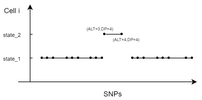 The numbers in brackets indicating the (alternative allele counts, total allele counts) aligned to the two SNP positions.
The inferred log likelihood can be expressed as:
\[ Logll_{inferred} = log(Trans_L)+log(dbinom(3,4,0.9))+log(dbinom(4,4,0.9))+log(Trans_R) \] The reversed log likelihood is then:
\[ Logll_{altered} = log(noTrans_L)+log(dbinom(3,4,0.1))+log(dbinom(4,4,0.1))+log(noTrans_R) \] Hence the logllRatio:
\[ logllRatio = Logll_{inferred} - Logll_{altered} \]
A larger logllRatio indicating we are more confident with the inferred Viterbi states for markers in the segment.
Diagnosic plots
The output files from sgcocaller can be directly parsed through readHapState function. However, we have a look at some cell-level metrics and segment-level metrics before we parse the sgcocaller output files.
Per cell QC
The function perCellQC generates cell-level metrics in a data.frame and the plots in a list.
We first identify the relevant file paths:
dataset_dir is the ouput directory from running sgcocaller and barcodeFile_path points to the file containing the list of cell barcodes.
suppressPackageStartupMessages({
  library(comapr)
  library(ggplot2)
  library(dplyr)
  library(Gviz)
  library(BiocParallel)
  library(SummarizedExperiment)
})
path_dir <- "/mnt/beegfs/mccarthy/scratch/general/Datasets/Hinch2019/"
dataset_dir <- paste0(path_dir,"output/sgcocaller/hinch/")
barcodeFile_path <-paste0(path_dir,"output/alignment/mergedBam/mergedAll.bam.barcodes.txt")We can locate the files and list the files to have a look:
list.files(path=dataset_dir)[1:5][1] "hinch_chr1_altCount.mtx" "hinch_chr1_snpAnnot.txt"
[3] "hinch_chr1_totalCount.mtx" "hinch_chr1_vi.mtx"
[5] "hinch_chr1_viSegInfo.txt" BiocParallel::register(BiocParallel::MulticoreParam(workers = 4))
#BiocParallel::register(BiocParallel::SerialParam())Running perCellChrQC function to find the cell-level statistics:
pcqc <- perCellChrQC("hinch",
                     chroms=paste0("chr",1:19),
                     path=dataset_dir,
                     barcodeFile=barcodeFile_path)
The generated scatter plots for selected chromosomes:
pcqc$plotWarning: Transformation introduced infinite values in continuous x-axis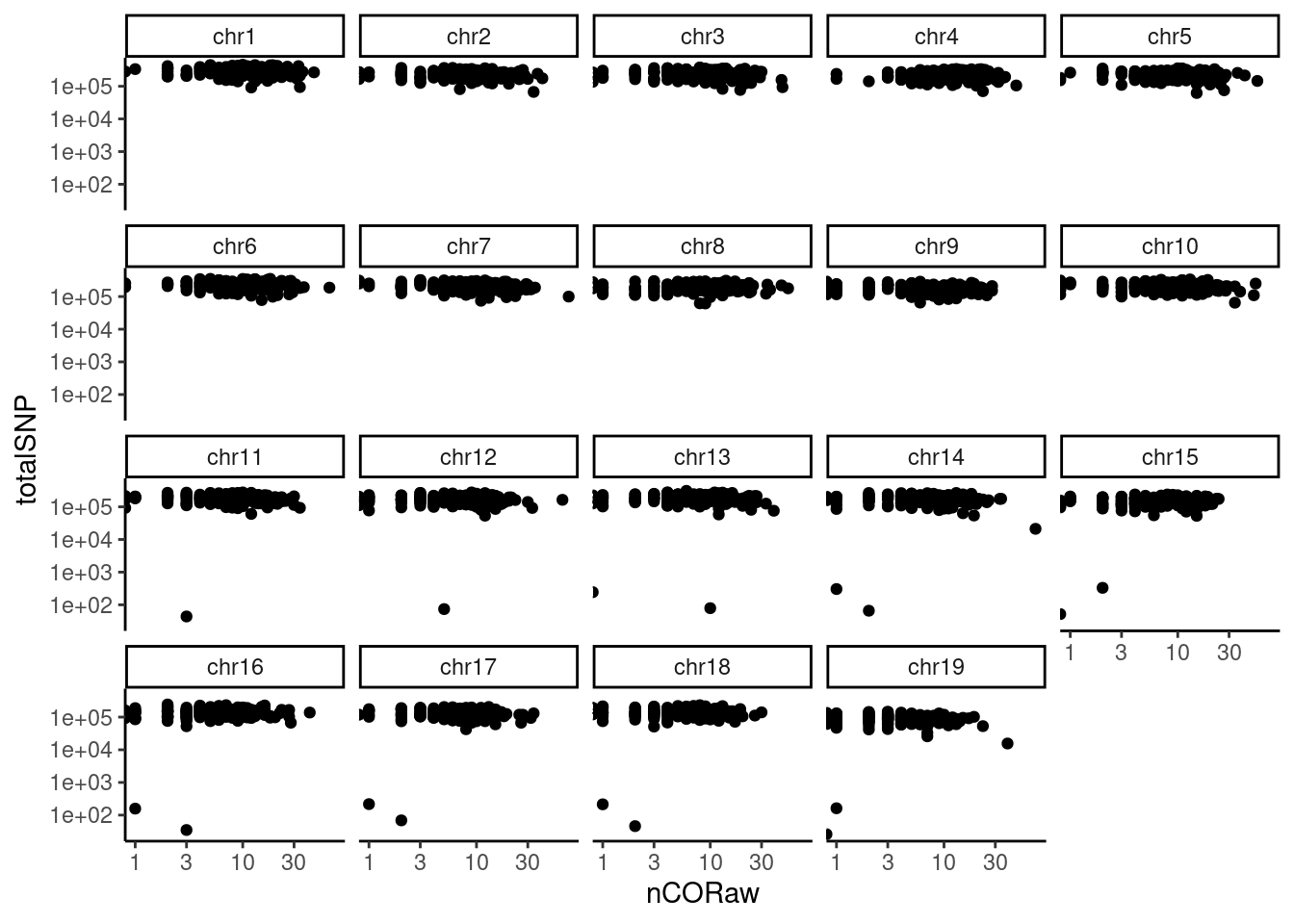
X-axis plots the number of haplotype transitions (nCORaw) for each cell and Y-axis plots the number of total SNPs detected in a cell. A large nCORaw might indicate the cell being a diploid cell included by accident or doublets. Cells with a lower totalSNPs might indicate poor cell quality.
A data.frame with cell-level metric is also returned:
pcqc$cellQC# A tibble: 3,686 × 4
Chrom totalSNP nCORaw barcode
<fct> <int> <dbl> <chr>
1 chr1 217857 22 SRR8454655
2 chr10 158079 27 SRR8454655
3 chr11 141643 10 SRR8454655
4 chr12 141169 3 SRR8454655
5 chr13 140556 17 SRR8454655
6 chr14 127778 16 SRR8454655
7 chr15 112856 5 SRR8454655
8 chr16 121926 6 SRR8454655
9 chr17 111465 6 SRR8454655
10 chr18 118538 8 SRR8454655
# … with 3,676 more rowsperSegChrQC
PerSegQC function visualises statistics of inferred haplotype state segments, which helps decide filtering thresholds for removing crossovers that do not have enough evidence by the data and the very close double crossovers which are biologically unlikely.
psqc <- perSegChrQC("hinch",chroms=paste0("chr",1),
                    path=dataset_dir,
                    barcodeFile=barcodeFile_path,
                    maxRawCO = 30)
psqc+theme_classic()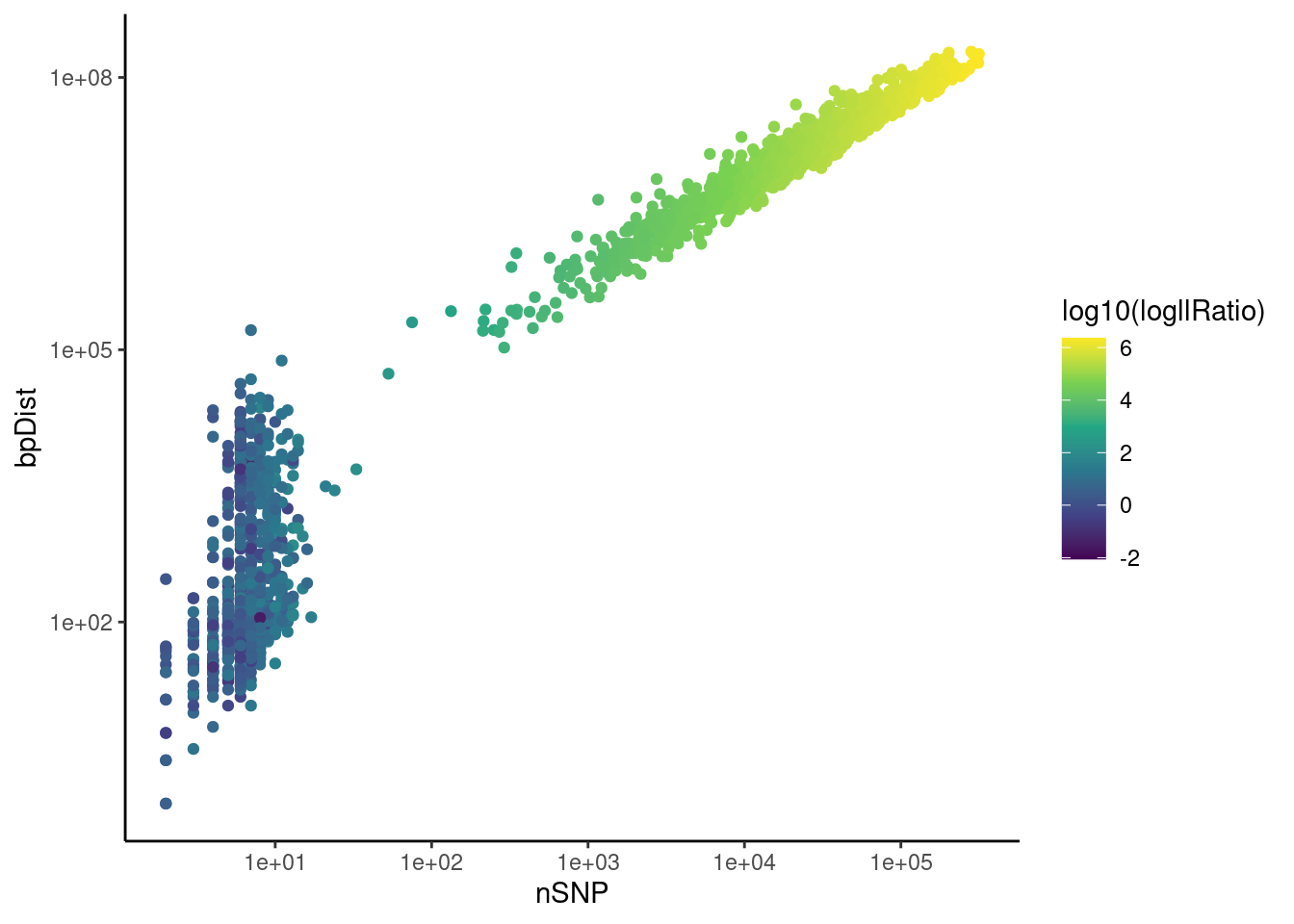
Parsing files using comapr
Now we have some idea about the features of this dataset, we can read in the files from sgcocaller which can be directly parsed through readHapState function. This function returns a RangedSummarizedExperiment object with rowRanges containing SNP positions that have ever contributed to crossovers in a cell, while colData contains the cell annotations such as barcodes.
The following filters have been applied:
- Segment level filters:
- minSNP=30, the segment that results in one/two crossovers has to have more than 30 SNPs of support
- minlogllRatio=150, the segment that results in one/two crossovers has to have logllRatio larger than 150.
- bpDist=1e5, the segment that results in one/two crossovers has to have base pair distances larger than 1e5
- Cell level filters:
- maxRawCO 55, the maximum number of raw crossovers (the number of state transitions from the _vi.mtx file) for a cell
- minCellSNP=200, there have to be more than 200 SNPs detected within a cell, otherwise this cell is removed.
BiocParallel::register(SerialParam())
hinch_rse <- readHapState(sampleName = "hinch",
                          path = dataset_dir,
                          chrom=paste0("chr",1:19),
                          barcodeFile = barcodeFile_path,
                          minSNP = 55, minCellSNP = 200,
                          maxRawCO = 20,
                          minlogllRatio = 150,
                          bpDist = 1e5)
#saveRDS(hinch_rse,file = "output/outputR/analysisRDS/hinch_rse.rds")BiocParallel::register(SerialParam())
hinch_rse <- readRDS(file="output/outputR/analysisRDS/hinch_rse.rds")The hinch_rse object:
hinch_rseclass: RangedSummarizedExperiment
dim: 33585 173
metadata(10): ithSperm Seg_start ... bp_dist barcode
assays(1): vi_state
rownames: NULL
rowData names(0):
colnames(173): SRR8454655 SRR8454656 ... SRR8454870 SRR8454871
colData names(1): barcodesThe rowRanges of hinch_rse
SummarizedExperiment::rowRanges(hinch_rse)GRanges object with 33585 ranges and 0 metadata columns:
seqnames ranges strand
<Rle> <IRanges> <Rle>
[1] chr1 3000258 *
[2] chr1 3001490 *
[3] chr1 3001712 *
[4] chr1 3001745 *
[5] chr1 3004324 *
... ... ... ...
[33581] chr19 61324579 *
[33582] chr19 61325233 *
[33583] chr19 61325919 *
[33584] chr19 61327767 *
[33585] chr19 61330760 *
-------
seqinfo: 19 sequences from an unspecified genome; no seqlengthsThe assay slot contains the Viterbi state matrix (SNP by Cell):
SummarizedExperiment::assay(hinch_rse)[1:5,1:5]5 x 5 sparse Matrix of class "dgCMatrix"
SRR8454655 SRR8454656 SRR8454657 SRR8454658 SRR8454660
[1,] . . . . .
[2,] . 2 . . .
[3,] . . . . .
[4,] 2 . . . .
[5,] . . . . .Note this matrix is more sparse which only contains the SNPs that contribute to crossovers in cells.
Samples group factor
We have sperm cells from only one individual in this dataset. However, to demonstrate the functions in comapr we split the cells into two groups.
## set the first 80 cells as group1 and rest as group2

colData(hinch_rse)$sampleGroup <- c(rep("Group1",ceiling(ncol(hinch_rse)/2)),rep("Group2",ncol(hinch_rse)-ceiling(ncol(hinch_rse)/2)))

colData(hinch_rse)
DataFrame with 173 rows and 2 columns
barcodes sampleGroup
<character> <character>
SRR8454655 SRR8454655 Group1
SRR8454656 SRR8454656 Group1
SRR8454657 SRR8454657 Group1
SRR8454658 SRR8454658 Group1
SRR8454660 SRR8454660 Group1
... ... ...
SRR8454863 SRR8454863 Group2
SRR8454864 SRR8454864 Group2
SRR8454867 SRR8454867 Group2
SRR8454870 SRR8454870 Group2
SRR8454871 SRR8454871 Group2Note combineHapState can be applied of there are multiple sets of outputs from sgcocaller.
Count crossovers in cells
The function countCOs can then be executed to find the crossover intervals and the number of crossovers for each cell within each crossover interval.
hinch_co_counts <- countCOs(hinch_rse)The SNP intervals list in the rowRanges slot:
rowRanges(hinch_co_counts)GRanges object with 2534 ranges and 0 metadata columns:
seqnames ranges strand
<Rle> <IRanges> <Rle>
[1] chr1 13416240-13419295 *
[2] chr1 18858161-18861351 *
[3] chr1 20068925-20069169 *
[4] chr1 25464178-25472637 *
[5] chr1 28213896-28218311 *
... ... ... ...
[2530] chr19 60044638-60047624 *
[2531] chr19 60069152-60070536 *
[2532] chr19 60070538-60070663 *
[2533] chr19 60070665-60074988 *
[2534] chr19 60373837-60375859 *
-------
seqinfo: 19 sequences from an unspecified genome; no seqlengthsThe assay slot of hinch_co_counts contains the number of crossovers per cell per SNP interval:
assay(hinch_co_counts)[1:5,1:5]DataFrame with 5 rows and 5 columns
SRR8454655 SRR8454656 SRR8454657 SRR8454658 SRR8454660
<numeric> <numeric> <numeric> <numeric> <numeric>
1 0 0 0 0 0
2 0 0 0 0 0
3 0 0 0 0 1
4 0 0 0 0 0
5 0 0 0 0 0mean(colSums(as.matrix(assay(hinch_co_counts))))[1] 12.03468Plot crossover counts
To get the number of crossovers per sperm cell, we just need to sum each column of the matrix in the assay slot. And the plotCount function plots the number of crossovers for each sperm.
plotCount(hinch_co_counts)+theme_classic()+
  scale_color_manual(values = c("all"="red"))+theme_classic(base_size = 25)+
  theme(axis.text = element_text(size = 25),
        axis.title = element_text(size =25),
        legend.position = "none",
          axis.text.x = element_blank(),
  axis.ticks.x = element_blank())+ylab("Crossover counts")+xlab("Mouse sperm cells")
Scale for 'colour' is already present. Adding another scale for 'colour',
which will replace the existing scale.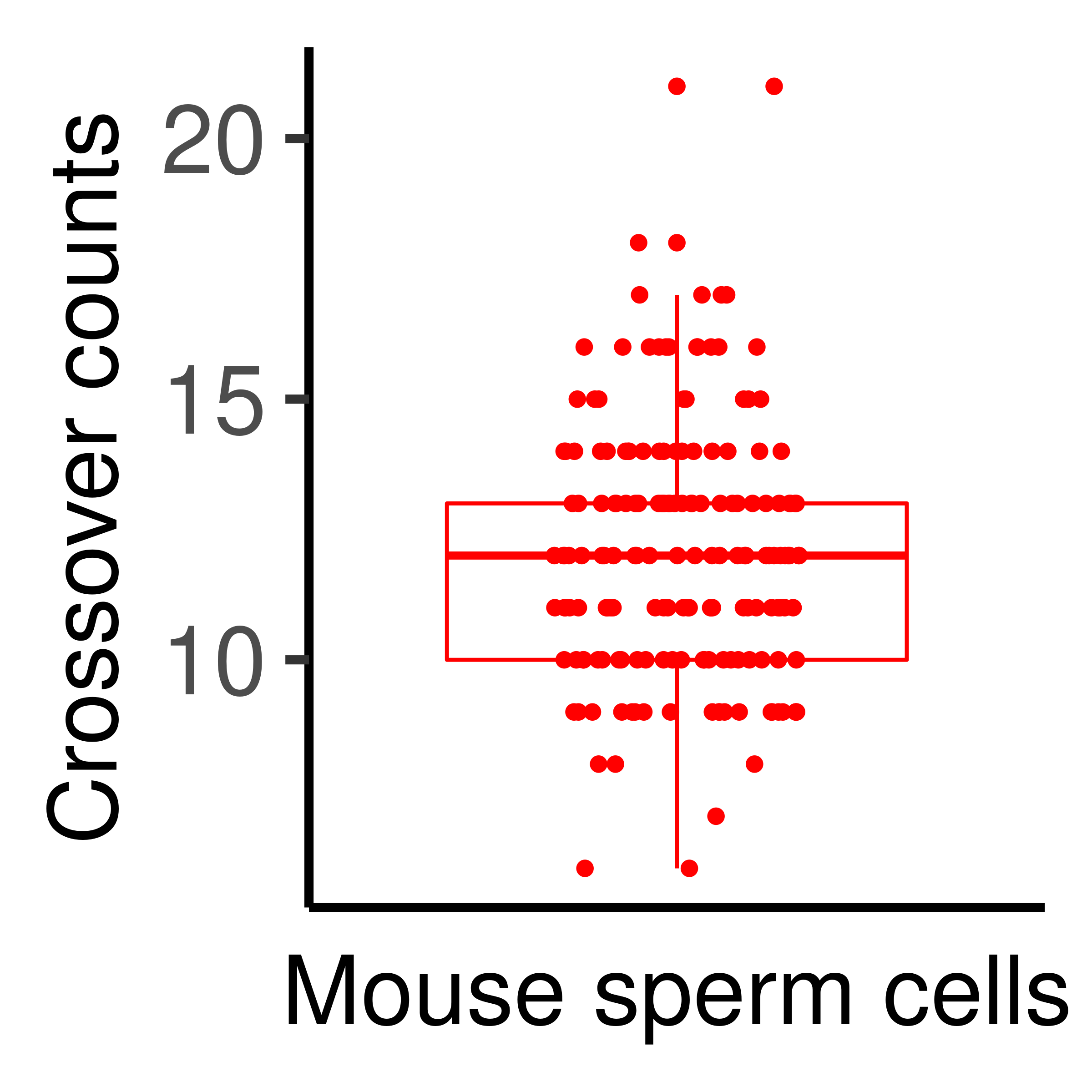
Or we can plotCount for each sample group:
plotCount(hinch_co_counts, group_by = "sampleGroup")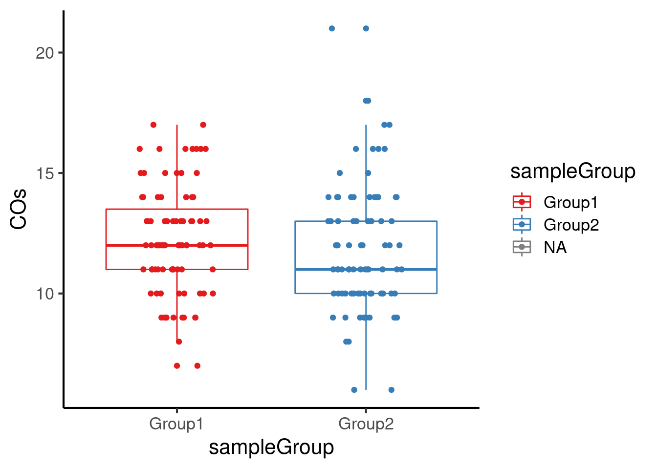
In addition, we can also plot the number of crossovers per chromosome (with mean number of crossovers and standard error bar):
plotCount(hinch_co_counts, ,by_chr = TRUE)+
  theme(axis.text.x = element_text(angle=90))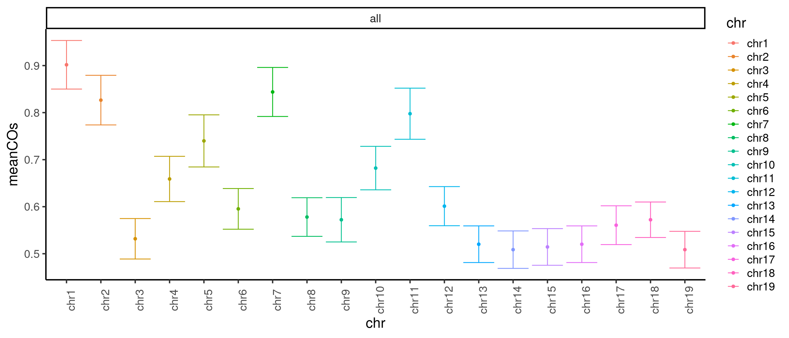
We can also generate bar plot counts of number of crossovers for each chromosome. We can see that for fewer double crossovers were called for smaller chromosomes.
plotCount(hinch_co_counts,by_chr = TRUE,
          plot_type ="hist")+theme_classic(base_size = 22)+facet_wrap(.~chr,ncol=8)
`stat_bin()` using `bins = 30`. Pick better value with `binwidth`.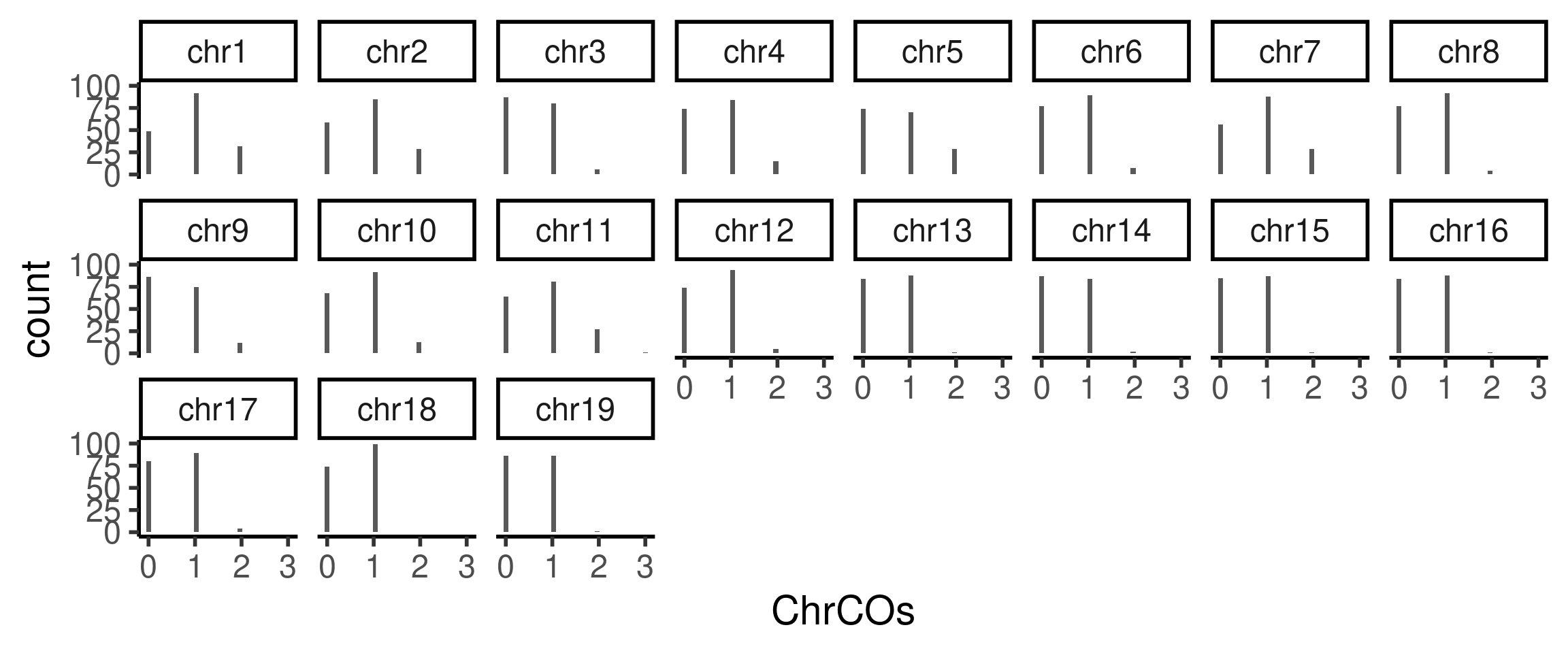
Plot SNP density track
The informative SNP markers’ distributions along the chromosome affects the crossover resolutions, therefore it is helpful to visualize the SNP density distribution.
We can generate the SNP density DataTrack with function getSNPDensityTrack which returns a DataTrack object from Gviz package.
## log=TRUE, the result after aggregation is returned on a log10 scale

snp_track_chr10 <- getSNPDensityTrack(chrom = "chr10",
                                      path_loc = dataset_dir,
                                      sampleName = "hinch",
                                      nwindow = 80,
                                      log = TRUE,
plot_type = "hist")plotTracks(snp_track_chr10)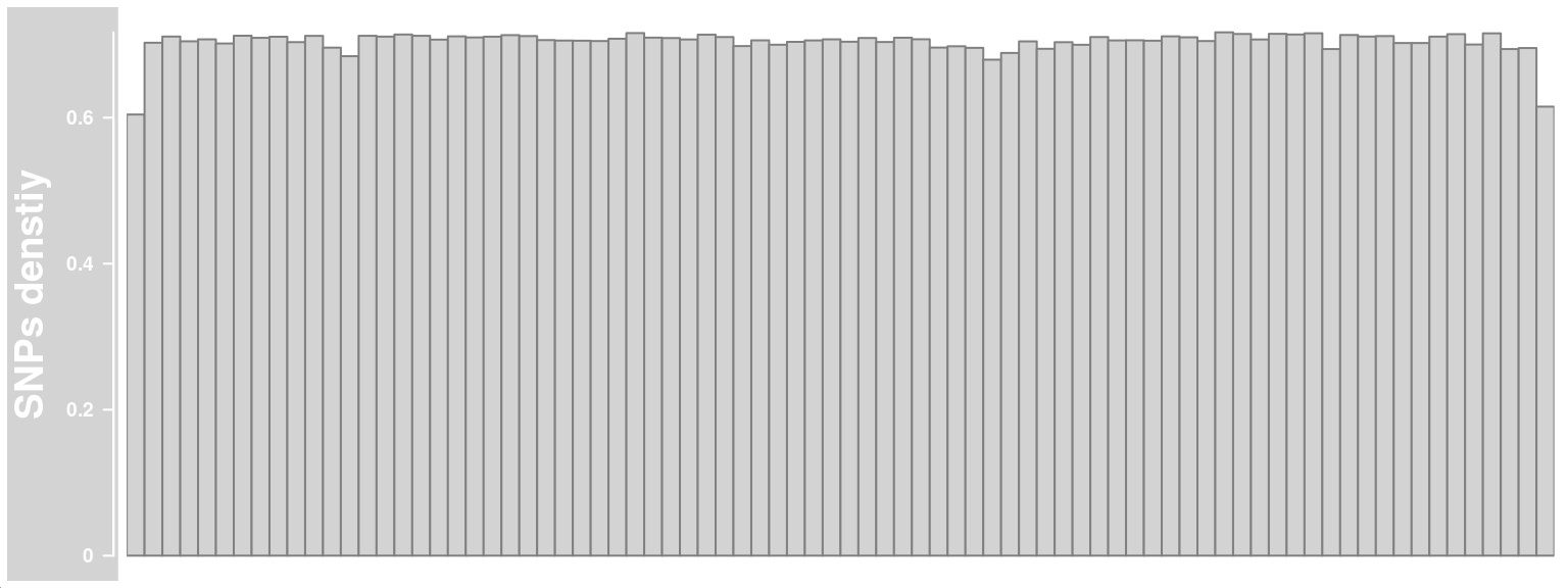
snp_track_chr10 <- setPar(snp_track_chr10,"cex.axis",1.5)Note that the behaviour of the 'setPar' method has changed. You need to reassign the result to an object for the side effects to happen. Pass-by-reference semantic is no longer supported.To change visualisation parameters we can use setPar:
snp_track_chr10 <- setPar(snp_track_chr10,"background.title","firebrick")Note that the behaviour of the 'setPar' method has changed. You need to reassign the result to an object for the side effects to happen. Pass-by-reference semantic is no longer supported.plotTracks(snp_track_chr10)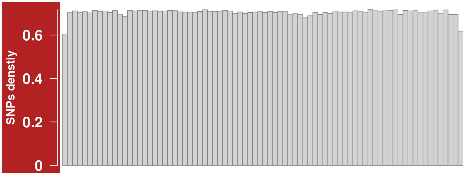
Change aggregation function to “sum”
snp_track_chr10 <- setPar(snp_track_chr10,"aggregation","sum")Note that the behaviour of the 'setPar' method has changed. You need to reassign the result to an object for the side effects to happen. Pass-by-reference semantic is no longer supported.plotTracks(snp_track_chr10)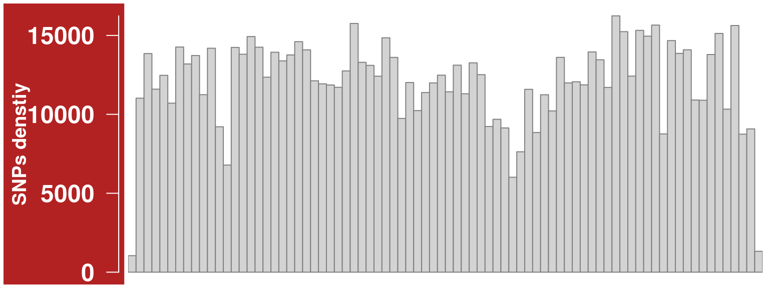
Plot Mean DP (read depth) across cells for each chromosome
meanDP_track_chr10 <- getMeanDPTrack(chrom = "chr10",
                            path_loc = dataset_dir,
                            nwindow = 80,
                            sampleName ="hinch",
                            barcodeFile=barcodeFile_path,
                            plot_type = "hist",
                            selectedBarcodes = colnames(hinch_co_counts),
                            snp_track = snp_track_chr10,
log =TRUE)plotTracks(meanDP_track_chr10)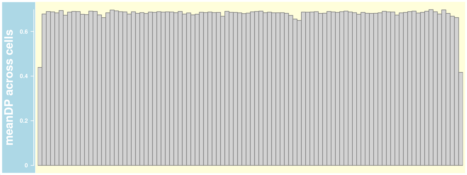
Visulise the raw Alternative Frequency (AF) plot with crossover region highlighted
for the selected cell
We can select a cell and visulise the raw Alternative Frequency (AF) plot with the called crossover region highlighted.
cell_af <- getCellAFTrack(chrom = "chr10",
               path_loc = dataset_dir,
               sampleName = "hinch",
               barcodeFile = barcodeFile_path,
               nwindow = 80,
               snp_track = snp_track_chr10,
               cellBarcode = colnames(hinch_co_counts)[1],
               co_count = hinch_co_counts,
               chunk = 8000L)
Generate a Highlight track with the returned list object cell_af
changed_bgcolor <- cell_af$af_track
changed_bgcolor <- setPar(changed_bgcolor, "background.title","#4C5270")
Note that the behaviour of the 'setPar' method has changed. You need to reassign the result to an object for the side effects to happen. Pass-by-reference semantic is no longer supported.ht <- HighlightTrack(changed_bgcolor,
range = cell_af$co_range[seqnames(cell_af$co_range)=="chr10"],
chromosome = "chr10")
plotTracks(ht,cex = 1.5)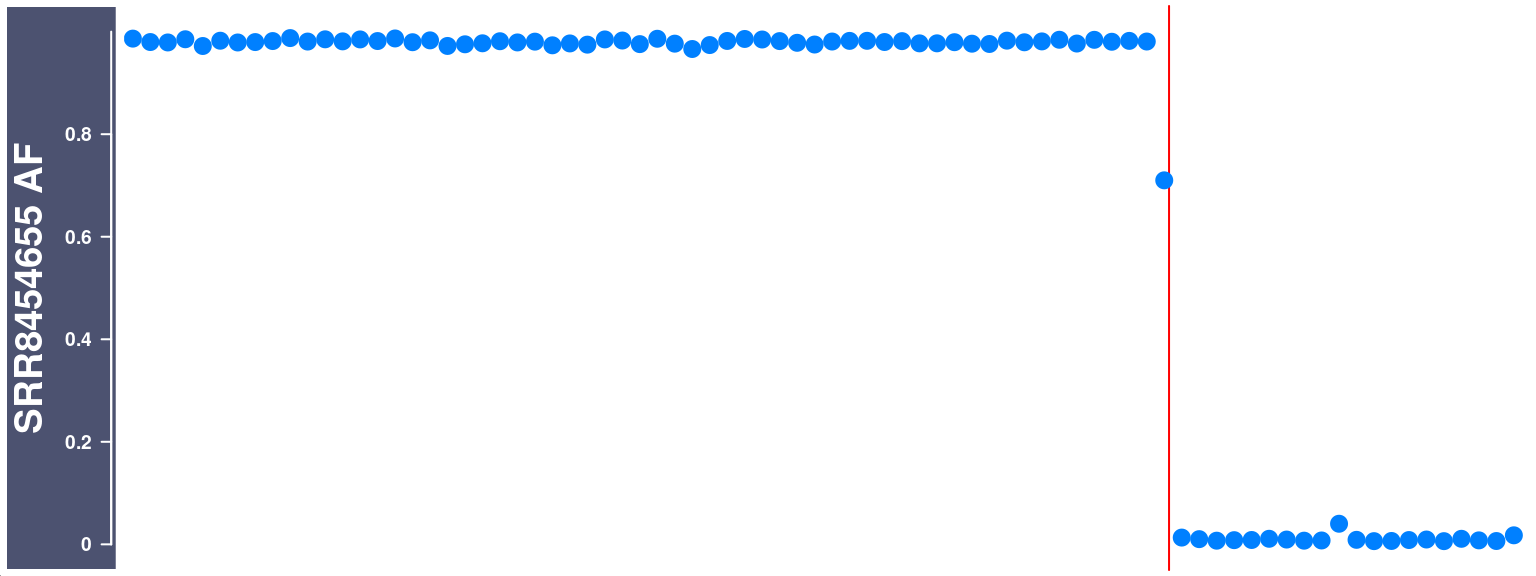
Easily combined with GenomeAxisTrack and IdeogramTrack
gtrack <- GenomeAxisTrack()
chr10_ideo <- IdeogramTrack(genome = "mm10", chromosome = "chr10")
plotTracks(list(chr10_ideo,gtrack, ht),cex.title = 1.2,
           cex.axis = 1.5,cex = 1.5)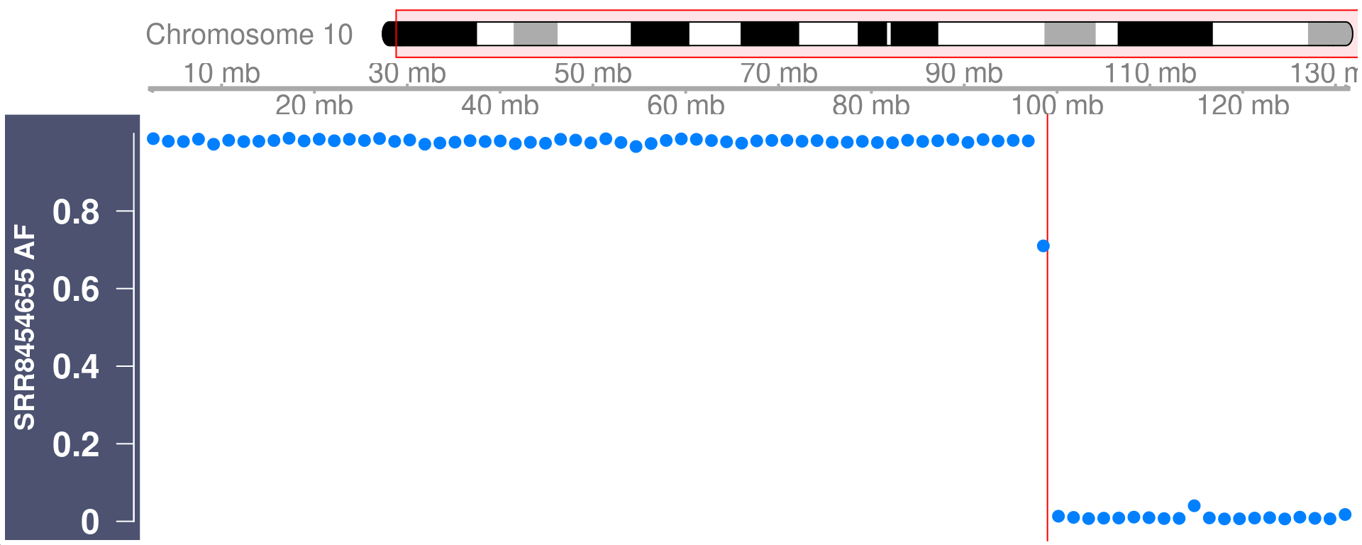
Plot SNP density along with crossover counts
While one can get the DataTracks for the AF and the called crossover regions of a set of cells with getAFTracks, comapr also offers the function for plotting crossover counts for each cell or averaged crossover counts across sample groups.
crossover_count_track <- DataTrack(range = rowRanges(hinch_co_counts),
                       genome = "mm10",
                       data = data.frame(assay(hinch_co_counts)),
                       name = "expected crossover counts across SNP intervals",
                       type = "heatmap",
                       groups = hinch_co_counts$sampleGroup,
                       col = c("red","blue"),
                       #aggregateGroups = TRUE,
                       aggregation = mean,
                       window =80)

plotTracks(list(gtrack,snp_track_chr10,crossover_count_track),
           chromosome = "chr10")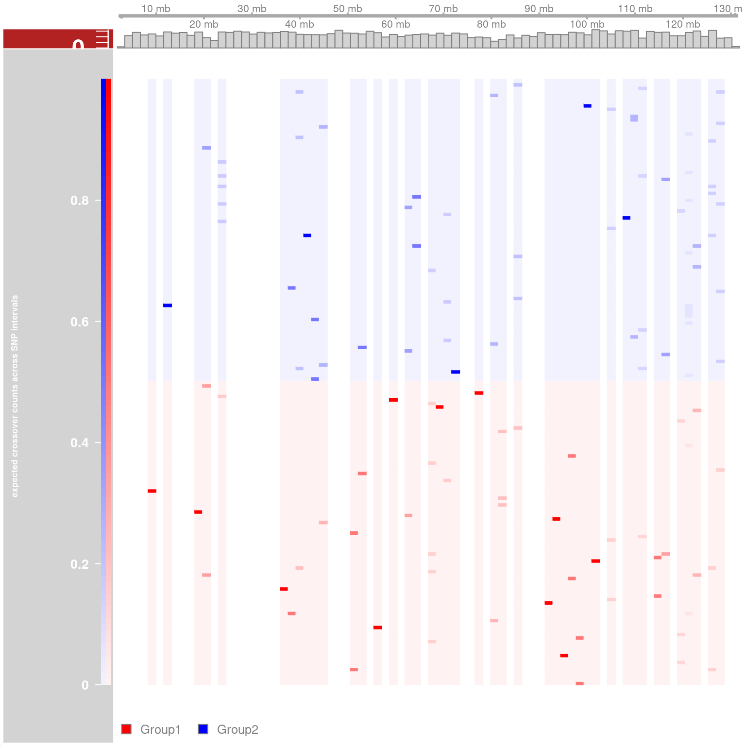
Chromosome 10
gtrack <- GenomeAxisTrack(cex=1.5)
snp_track_chr10 <- setPar(snp_track_chr10,"cex.axis",1.5)
Note that the behaviour of the 'setPar' method has changed. You need to reassign the result to an object for the side effects to happen. Pass-by-reference semantic is no longer supported.snp_track_chr10 <- setPar(snp_track_chr10,"cex.title",1.5)Note that the behaviour of the 'setPar' method has changed. You need to reassign the result to an object for the side effects to happen. Pass-by-reference semantic is no longer supported.#plotTracks(snp_track_chr10)
crossover_count_track <- DataTrack(range = rowRanges(hinch_co_counts),
genome = "mm10",
data = data.frame(assay(hinch_co_counts)),
name = "Mean\ncrossovers",
type = c("heatmap"),
groups = hinch_co_counts$sampleGroup,
col = c("red","blue"),
aggregateGroups = TRUE,
aggregation = mean,
window =80,cex.title=1.5,
cex.axis =1.5,
background.title = "#F652A0")
plotTracks(list(gtrack,snp_track_chr10,crossover_count_track),
chromosome = "chr10",sizes = c(1,2,2),window =50)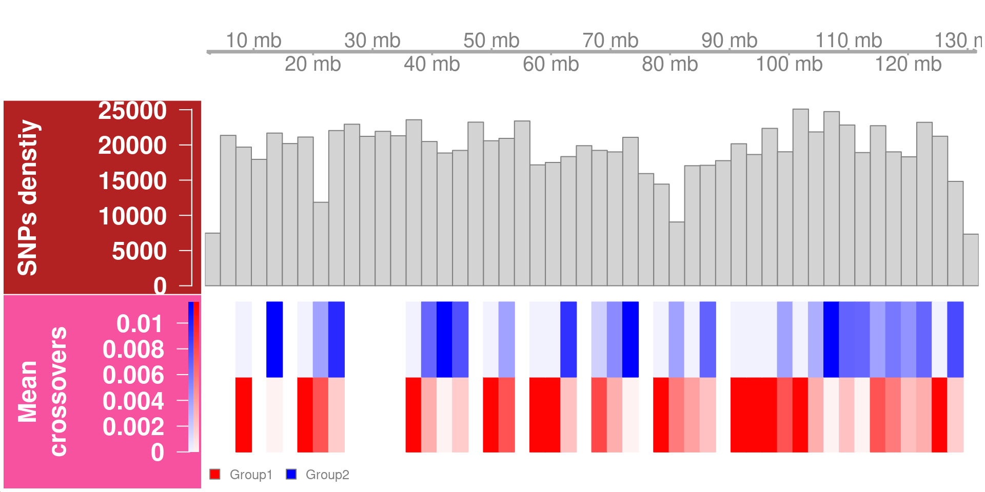
Chromosome 1
snp_track_chr1 <- getSNPDensityTrack(chrom = "chr1",
                                      path_loc = dataset_dir,
                                      sampleName = "hinch",
                                      nwindow = 80,
                                      log = FALSE,
                                      plot_type = "hist")

snp_track_chr1 <- setPar(snp_track_chr1,"background.title","firebrick")
Note that the behaviour of the 'setPar' method has changed. You need to reassign the result to an object for the side effects to happen. Pass-by-reference semantic is no longer supported.plotTracks(list(gtrack,snp_track_chr1,crossover_count_track),
chromosome = "chr1")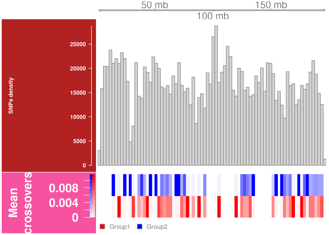
| Version | Author | Date |
|---|---|---|
| 3883a5d | rlyu | 2022-01-10 |
Calculate Genetic distances from crossover rates
The raw crossover rates estimated from observed crossovers across SNP intervals for a group of samples are commonly converted into genetic distances in units of centiMorgans via mapping functions such as the Kosambi or the Haldane function.
Haldane, cM =−0.5×ln(1−2r)×100,
Kosambi, cM=0.25×ln ((1+2r)/(1−2r))×100,
where r is the recombination fraction.
The Haldane mapping function adds mathematical adjustments to the recombination fraction. It assumes that crossover events are random and independent along the chromosome, and the number of crossover events between two loci follows a Poisson distribution. Haldane’s mapping function adjusts underestimated crossover rate in larger intervals that are likely to have unobserved even number of crossovers. Kosambi’s mapping function was derived based on Haldane’s and takes consideration of crossover interference.
We can calculate the genetic distances with the sperm dataset using calGeneticDist function:
# mapping_fun = "k" for applying the kosambi function

hinch_dist <- calGeneticDist(hinch_co_counts,
                             mapping_fun = "k")
The total genetic distances across the autosomes are then:
sum(rowData(hinch_dist)$kosambi)[1] 1203.548The genetic distances can also be calculated per sample group. It is useful for doing comparative analysis. We can also supply a bin_size parameter to get the genetic distances calcuated on binned chromosome intervals.
hinch_dist_groups <- calGeneticDist(hinch_co_counts,
                                    group_by = "sampleGroup",
                                    bin_size = 1e7)
The genetic distances per group can be derived as:
Matrix::colSums(as.matrix(mcols(hinch_dist_groups))) Group1 Group2
1225.525 1181.623 Plot genetic distances
The genetic distances across chromosome bins can be visualized by plotGeneticDist function:
plotGeneticDist(hinch_dist_groups,chr = "chr10")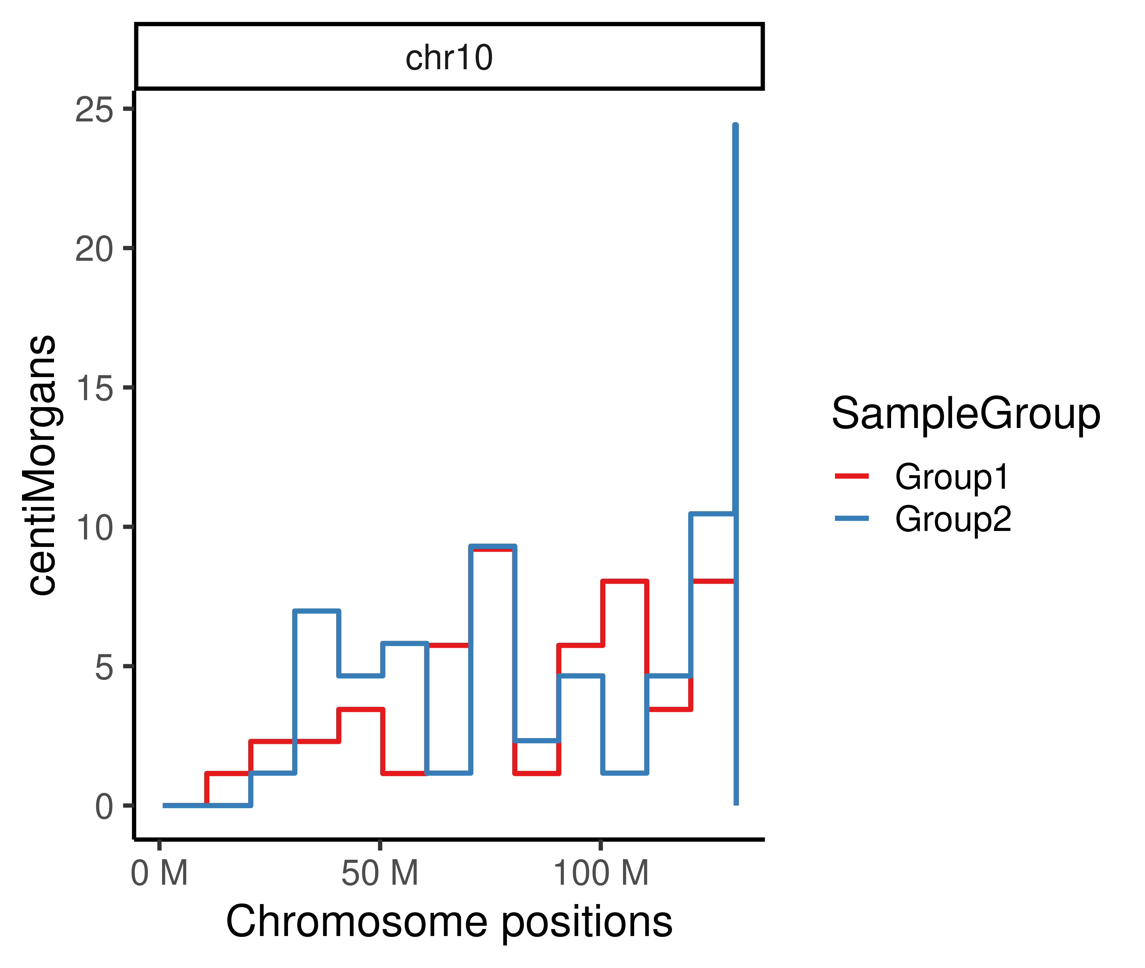
plotGeneticDist(hinch_dist_groups,chr = "chr1")+theme_classic(base_size = 25)+
  scale_color_manual(values = c("Group1"="#122620",
                                "Group2" = "#D6AD60" ))+
  theme(legend.position = "top",
        plot.margin=margin(t =  0.5, r = 1.5, b = 0, l = 0.5, unit = "cm"))+
  ylab("CentiMorgans per 10 Mb")
Scale for 'colour' is already present. Adding another scale for 'colour',
which will replace the existing scale.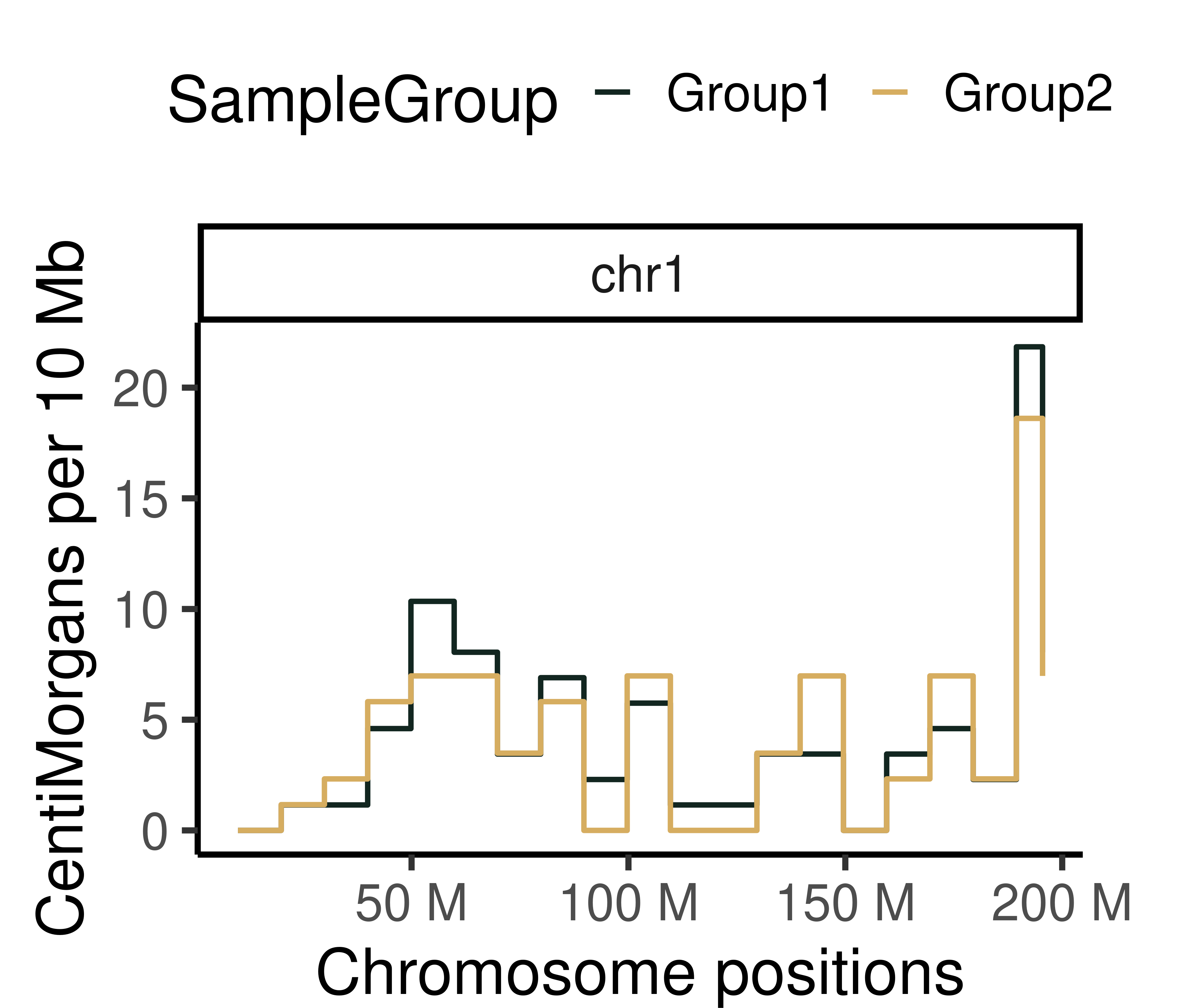
hinch_dist_groups_non_bin <- calGeneticDist(hinch_co_counts,
                                            group_by = "sampleGroup")
hinch_dist_groups_non_bin_gr <- rowRanges(hinch_dist_groups_non_bin)
mcols(hinch_dist_groups_non_bin_gr) <- mcols(hinch_dist_groups_non_bin_gr)$kosambi

plotGeneticDist(hinch_dist_groups_non_bin_gr,chr = "chr1",cumulative = TRUE)+
  theme_classic(base_size = 25)+
  theme(legend.position = "none",
                plot.margin=margin(t =  0.5, r = 1.5, b = 0, l = 0.5, unit = "cm"))+
  scale_color_manual(values = c("Group1"="#122620",
                                "Group2" = "#D6AD60" ))+
  ylab("Cumulative\ncentiMorgans")
Scale for 'colour' is already present. Adding another scale for 'colour',
which will replace the existing scale.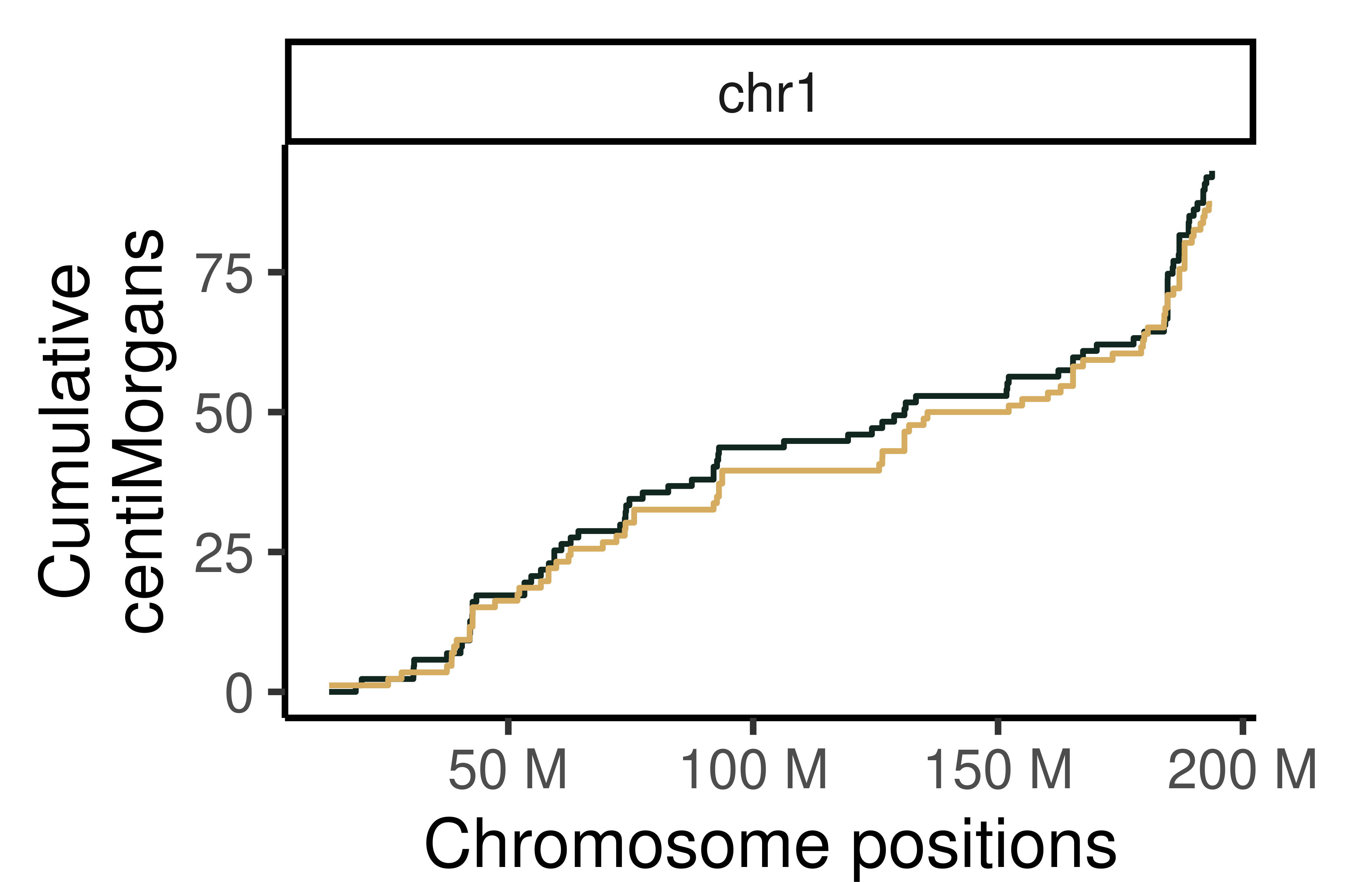
non_group_gr <- calGeneticDist(hinch_co_counts,bin_size = 1e7)
#mcols(non_group_gr) <- mcols(non_group_gr)$kosambi
colnames(mcols(non_group_gr)) <- "allCells"

plotGeneticDist(non_group_gr,chr = "chr1")+theme_classic(base_size = 25)+
  theme(legend.position = "none",
        plot.margin=margin(t =  0.5, r = 1.5, b = 0, l = 0.5, unit = "cm"))+
  scale_color_manual(values =c("allCells" = "darkblue"))+ylab("CentiMorgans per 10 Mb")
Scale for 'colour' is already present. Adding another scale for 'colour',
which will replace the existing scale.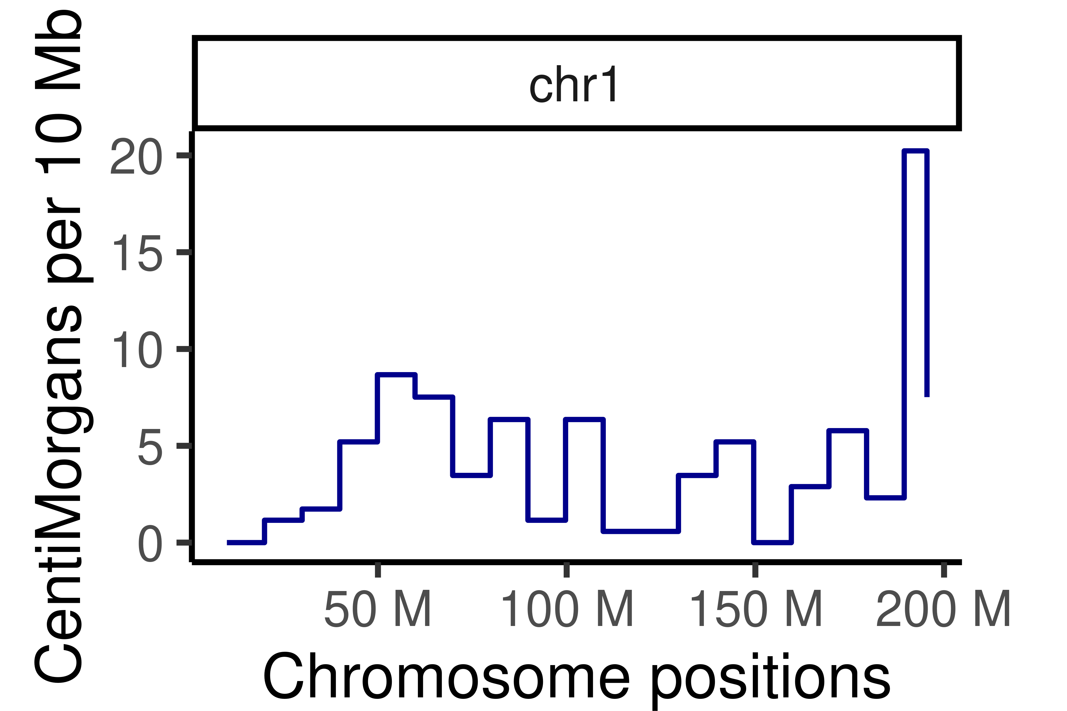
plotGeneticDist(hinch_dist_groups,chr = c("chr1","chr2"))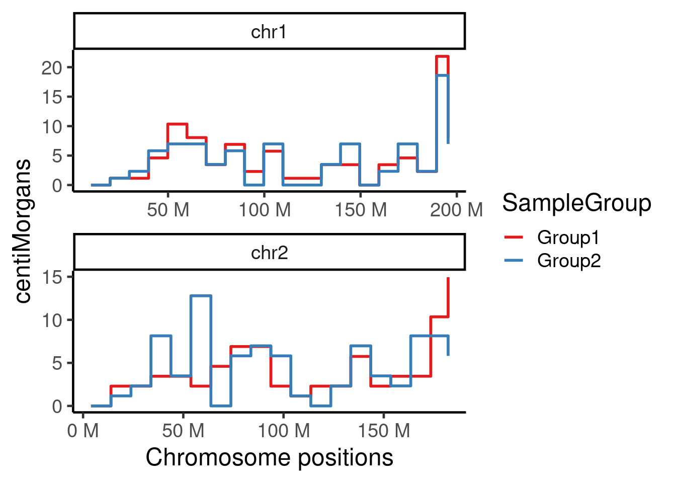
| Version | Author | Date |
|---|---|---|
| 3883a5d | rlyu | 2022-01-10 |
plotGeneticDist(hinch_dist_groups,chr = c("chr15","chr16"))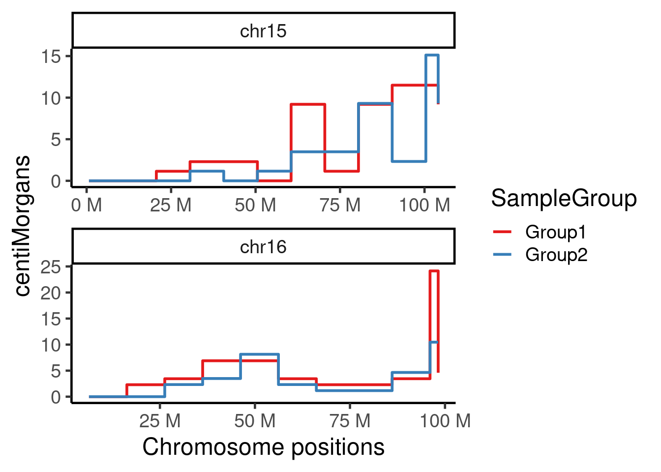
| Version | Author | Date |
|---|---|---|
| 3883a5d | rlyu | 2022-01-10 |
We can also do cumulative centiMorgans plots and the whole genome plot:
plotGeneticDist(hinch_dist_groups,chr = c("chr15","chr16"),cumulative = TRUE)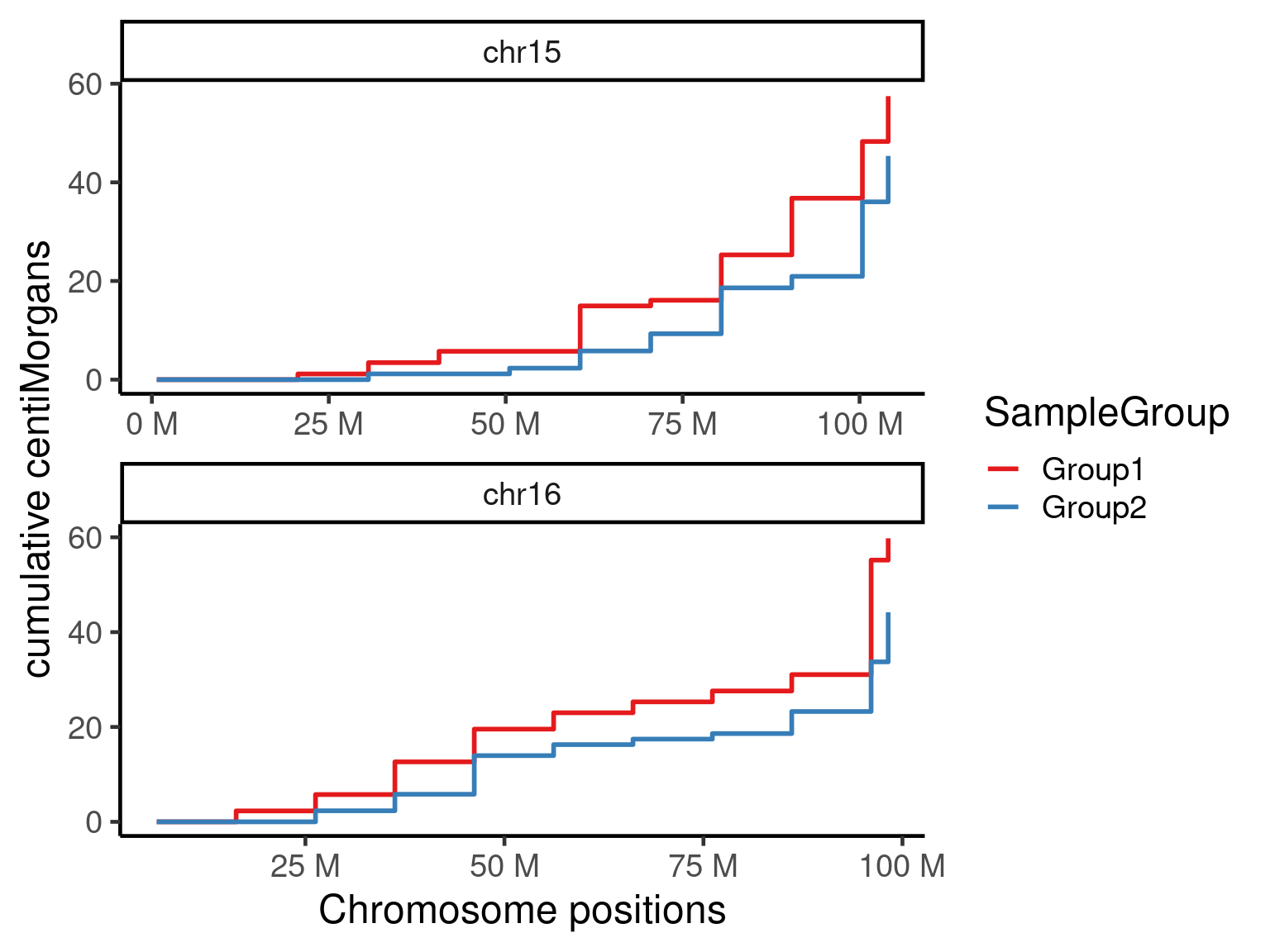
plotWholeGenome(hinch_dist_groups)+theme_classic(base_size = 25)+
  theme(axis.text.x = element_text(angle = 90),
        legend.position = "none")+
  scale_color_manual(values = c("Group1"="#122620",
                                "Group2" = "#D6AD60" ))+xlab("Cumulative whole genome")+
  ylab("Cumulative\ncentiMorgans")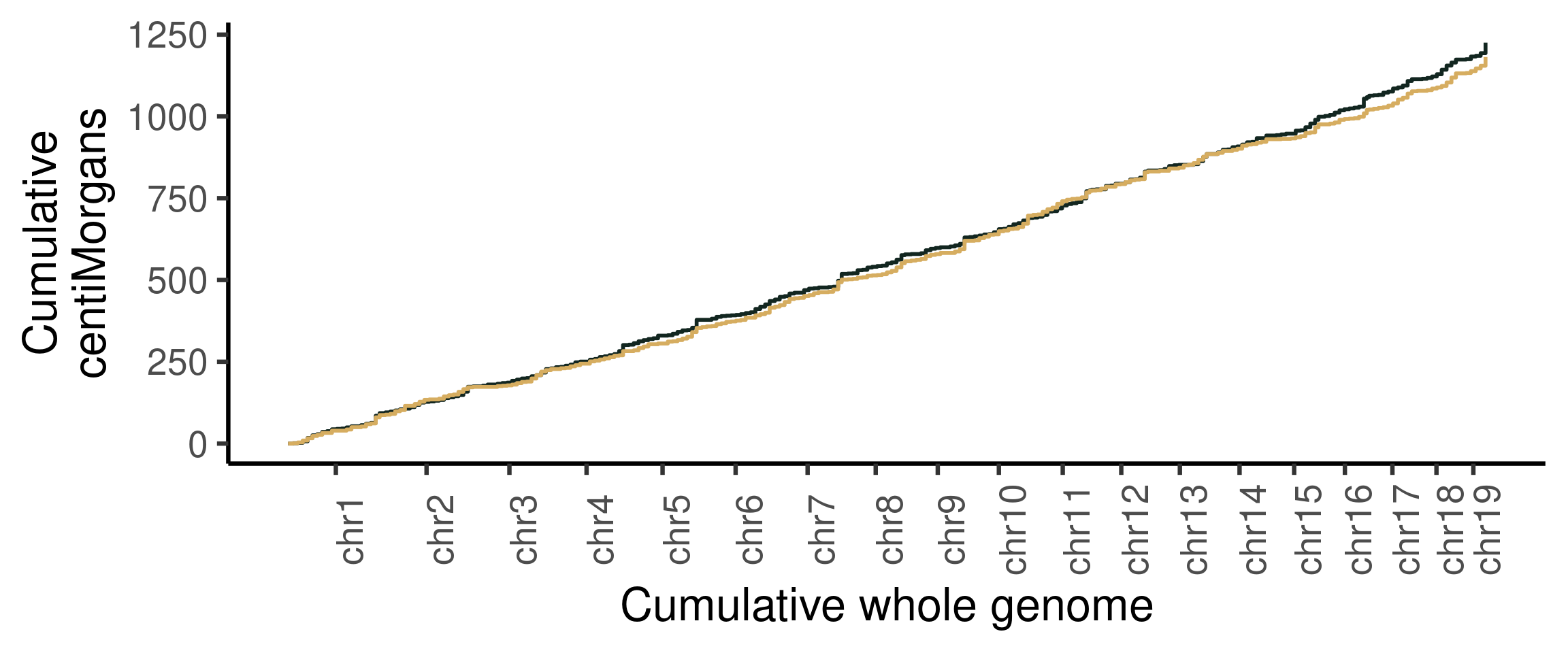
The two sample groups are similar by looking at the cumulative centiMorgan growth curves of the two.
Group comparison
The calculated total genetic distances for the two groups show that Group1 has slightly larger total genetic distances resulted from more meiotic crossovers observed.
To test whether the observed difference is statistically significant, we can apply Bootstrapping test to get confidence intervals of group differences and permutation testing for calculating a significance level.
Bootstrapping
set.seed(100)
bootsResult <- bootstrapDist(hinch_co_counts,
                             group_by = "sampleGroup",
                             B = 2000)
The 95% confidence intervals for the group differences by bootstrapping is then:
quantile(bootsResult,c(0.025,0.975)) 2.5% 97.5%
-29.4546 116.5531 which includes zero thus the observed difference is not significant at level of 0.05.
The histogram of the bootstrapping results:
btrp_quantile <- quantile(bootsResult,c(0.025,0.975))
ggplot()+geom_histogram(mapping = aes(x = bootsResult),
                        fill = "#7c7b89")+theme_classic(base_size = 18)+
  geom_vline(mapping = aes(xintercept  = btrp_quantile[1],color = "2.5%"),size =1.5)+
  geom_vline(mapping = aes(xintercept  = btrp_quantile[2],
             color = "97.5%"),size =1.5)+
  scale_x_continuous(breaks = c( -100,-50,
                                 round(btrp_quantile[1],2),
                                 0  , 50 , 75 ,
                                round(btrp_quantile[2],2),
                                150,  200) ,
                     labels = c( -100,-50,
                                 round(btrp_quantile[1],2),
                                 0  , 50 , 75 ,
                                round(btrp_quantile[2],2),
                                150,  200))+
  xlab("Bootstrapping results")+
  theme_classic(base_size = 25)+
  scale_color_manual(values = c("97.5%"="#0b7fab","2.5%"="#e9723d"),
                     name = "Quantile")+ylab("Count")+
  theme(legend.position = "top",
        axis.text.x = element_text(angle = 90))
`stat_bin()` using `bins = 30`. Pick better value with `binwidth`.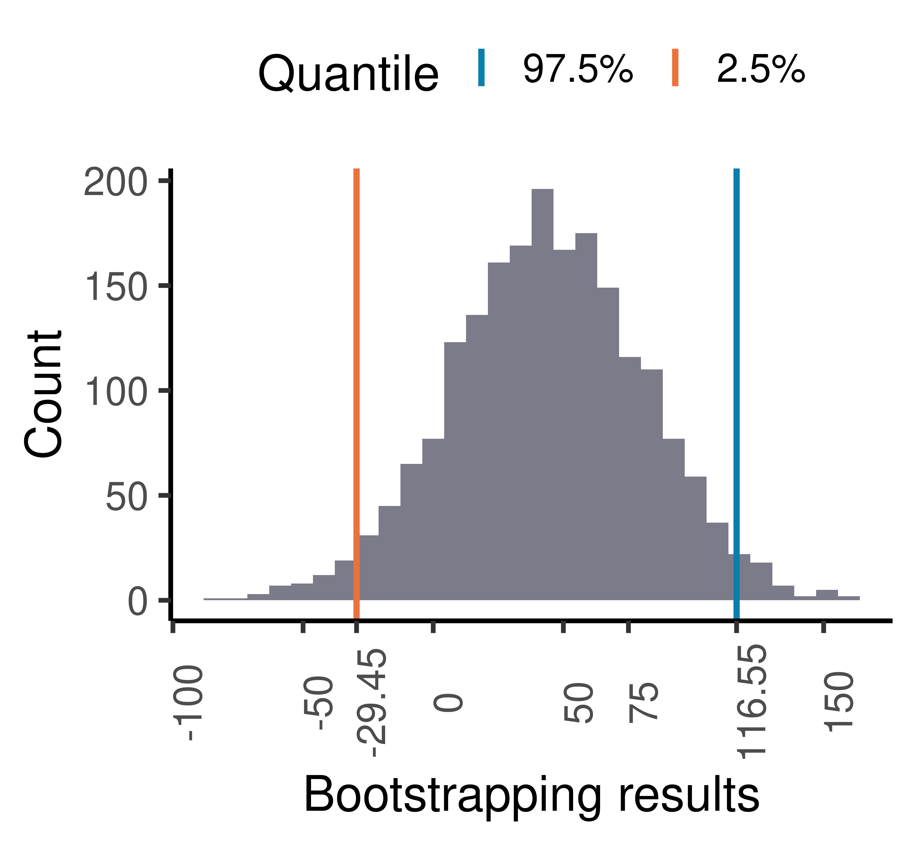
| Version | Author | Date |
|---|---|---|
| 3883a5d | rlyu | 2022-01-10 |
## seq(from = -100, to = 200, by = 50)dat <- with(density(bootsResult), data.frame(x, y))
ggplot(dat,mapping = aes(x = x,y=y))+geom_line(fill = "#7c7b89")+
geom_area(mapping = aes(x = ifelse(x > btrp_quantile[1] &
x < btrp_quantile[2],
x, NA)),
fill = "hotpink",alpha=0.3)+theme_classic()+
xlab("Bootstrapping results")Warning: Ignoring unknown parameters: fillWarning: Removed 253 rows containing missing values (position_stack).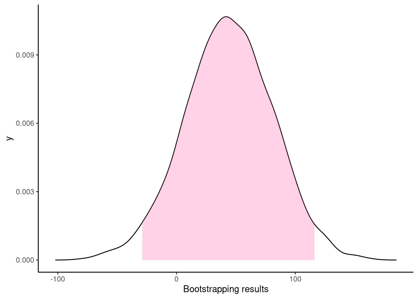
Permutation
We next apply permutation testing using the permuteDist function.
set.seed(2021)
BiocParallel::register(BiocParallel::SerialParam())
perms <- permuteDist(hinch_co_counts,group_by = "sampleGroup",
                     B=2000)
perms$observed_diff
[1] 43.90172perms$nSample[1] 87 86sum(is.na(perms$permutes))[1] 0We can then use the statmod::permp() function (Phipson and Smyth 2010) to calculate an exact p-value for this set of permutation results:
padjust <- statmod::permp(x = sum(perms$permutes> perms$observed_diff),
               nperm = 2000,
               n1 = perms$nSample[1],
               n2 = perms$nSample[2],
               twosided = F)
padjust
[1] 0.1149425We can see that the calculated p-value was not significant.
ggplot()+geom_histogram(mapping = aes(x = perms$permutes),
                        fill = "#7c7b89")+theme_classic()+
  geom_vline(mapping = aes(xintercept = perms$observed_diff,color ="observed difference"),
             size = 1.5,)+theme_classic(base_size = 25)+
  geom_text(mapping = aes(x= 108, y = 180,
                          label = paste0("p-value = ",round(padjust,2))),
            size = 7)+xlab("Permutation results")+
  scale_color_manual(values = c("observed difference"="black"),
                     name = "")+theme(legend.position = "top",
                                      axis.title.x = element_text(margin = margin(t = 30, r = 20, b = 0, l = 0)))+ylab("Count")
`stat_bin()` using `bins = 30`. Pick better value with `binwidth`.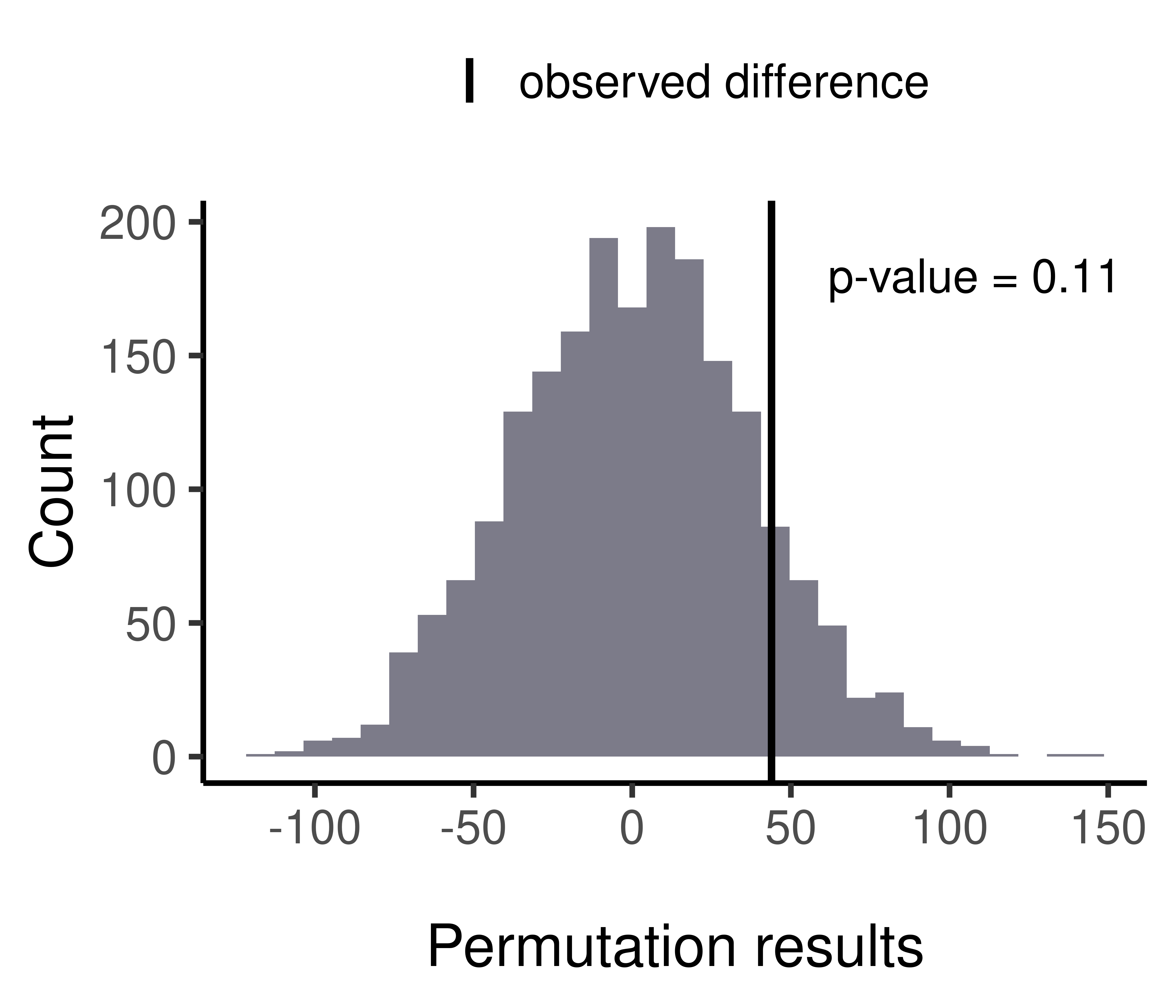
| Version | Author | Date |
|---|---|---|
| 3883a5d | rlyu | 2022-01-10 |
Filtered out sperm cells
During the first step of constructing the RangedSummarizedExperiment object, some cells were filtered out due to 1, some chromsomes having too few SNPs (<200), 2, some chromsomes have been called with excessive amount of crossovers. Too many crossovers were called (biologically impossiable) is likely due to “doublet” cells, i.e DNA reads from two sperm cells were regarded as one cell, or the sperm cell’s homologous chromosomes were not separated properly in meiosis. For this particular dataset, it is more likely due to the second case.
Plot alternative allele frequence tracks for chromsomes with excessive number
of crossovers
filteredCells <- read.table(file ="output/hinch_filtered_barcodes_doublets.txt",
                            header =T)
head(filteredCells)
Chrom totalSNP nCORaw barcode
1 chr10 249399 53 SRR8454765
2 chr12 163651 63 SRR8454806
3 chr6 187131 64 SRR8454806
4 chr8 177959 53 SRR8454806
5 chr5 145337 55 SRR8454823
6 chr10 109396 51 SRR8454677cell_af_chr10 <- getCellAFTrack(chrom = "chr10",
path_loc = dataset_dir,
sampleName = "hinch",
barcodeFile = barcodeFile_path,
nwindow = 300,
snp_track = snp_track_chr10,
cellBarcode = "SRR8454765",
co_count = hinch_co_counts,
chunk = 8000L)
cell_af_only <- cell_af_chr10$af_track
cell_af_only <- setPar(cell_af_only, "background.title","#4C5270")Note that the behaviour of the 'setPar' method has changed. You need to reassign the result to an object for the side effects to happen. Pass-by-reference semantic is no longer supported.Generate a Highlight track with the returned list object cell_af
ht <- HighlightTrack(cell_af_only,
                     range = cell_af_chr10$co_range[seqnames(cell_af_chr10$co_range)=="chr10"],
                     chromosome = "chr10")
plotTracks(ht)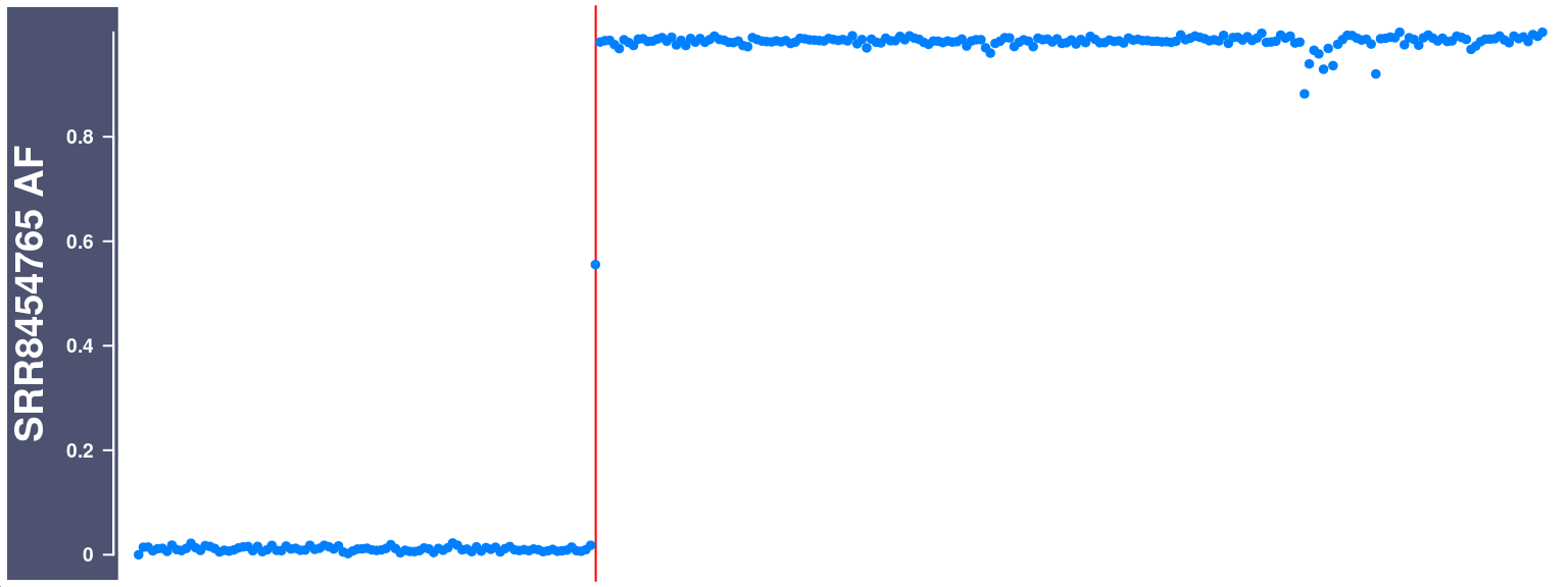
| Version | Author | Date |
|---|---|---|
| 3883a5d | rlyu | 2022-01-10 |
Match with crossovers called in the original paper
The cell’s crossover ranges can be found by getCellCORange function:
called_co_cell <- getCellCORange(co_count = hinch_co_counts,
                                 cellBarcode = colnames(hinch_co_counts)[1])
We now compare the crossovers called by ssocaller and comapr with the crossovers positions identified in the original paper (Hinch et al. 2019).
We first collect the crossover regions for each cell:
called_co_df <- lapply(colnames(hinch_co_counts), function(srr){

  called_co_cell <- getCellCORange(co_count = hinch_co_counts,
                                   cellBarcode = srr)
  called_co_df <- as.data.frame(called_co_cell)
  called_co_df$SRR <- srr
  called_co_df


})
called_co_df <- do.call("rbind",called_co_df)head(called_co_df) seqnames start end width strand SRR
1 chr2 152092358 152096706 4349 * SRR8454655
2 chr3 127265735 127268073 2339 * SRR8454655
3 chr5 100598558 100604496 5939 * SRR8454655
4 chr5 148434132 148435557 1426 * SRR8454655
5 chr6 39274873 39300625 25753 * SRR8454655
6 chr6 121425933 121426008 76 * SRR8454655called_co_df$chr <- called_co_df$seqnamesThe published crossover positions from (Hinch et al. 2019) was downloaded from GEO with GSE125326:
pub_co <- read.table(file ="references/publishedCrossovers.txt")
pub_co$chr <- paste0("chr",pub_co$chr)
pub_co <- pub_co[pub_co$chr!="chrX",]
merged_df <- merge(called_co_df, pub_co, by.x =c("SRR","chr"),
                   suffixes = c(".called",".pub"))
The number of crossovers called for each cell are highly concordant. The differences in number of crossovers called per cell are plotted in histogram down below. and we can see that our approach is more conservative. However, one can adjust the filtering thresholds mentioned at the start of this section to be less conservative.
sgcocaller_cos <- called_co_df %>% group_by(SRR) %>% summarise(COs_sgcocaller = n())

hinch_cos <- pub_co %>% group_by(SRR) %>% summarise(COs_hinch = n())

sgcocaller_cos %>% left_join(hinch_cos) %>%
  ggplot()+geom_histogram(mapping =
                            aes(x= (COs_sgcocaller - COs_hinch)))+theme_classic()
Joining, by = "SRR"`stat_bin()` using `bins = 30`. Pick better value with `binwidth`.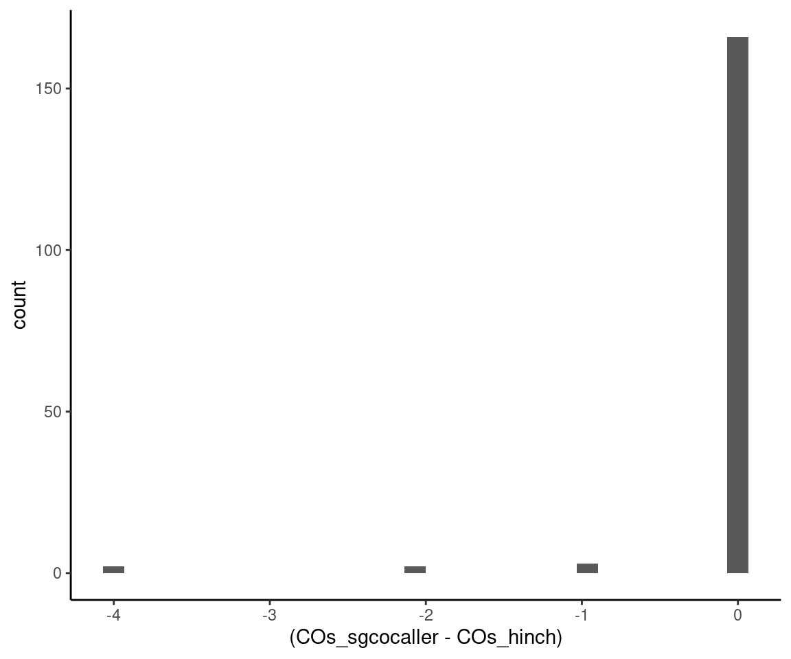
Differences in number of crossovers called by the two methods
sgcocaller_cos %>% left_join(hinch_cos) %>%
  ggplot()+geom_jitter(mapping =
                            aes(x= (COs_sgcocaller - COs_hinch), y ="diff"),
                       width = 0.3)+
  theme_classic()
Joining, by = "SRR"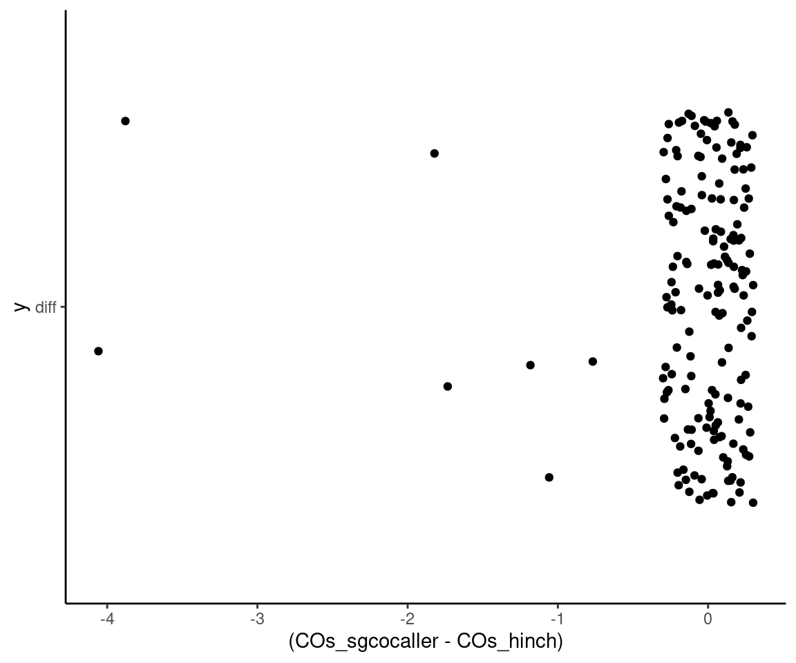
Differences in number of crossovers called by the two methods
sgcocaller_cos %>% left_join(hinch_cos) %>%
  mutate(diff = as.character(abs(COs_sgcocaller-COs_hinch))) %>% ggplot()+
  geom_jitter(mapping = aes(x = COs_sgcocaller,
                            y= COs_hinch,
                            color = diff,shape = diff),size =2.5)+
  theme_classic(base_size = 25)+scale_colour_viridis_d()+ylab("COs_published")+
  # scale_color_manual(
  #   values = c("0"="#58c8c9","1"="#48a3a4","2"="#367a7a","4"="#235050"))+
  theme(legend.position = c(0.5, 1),
          legend.direction = "horizontal")
Joining, by = "SRR"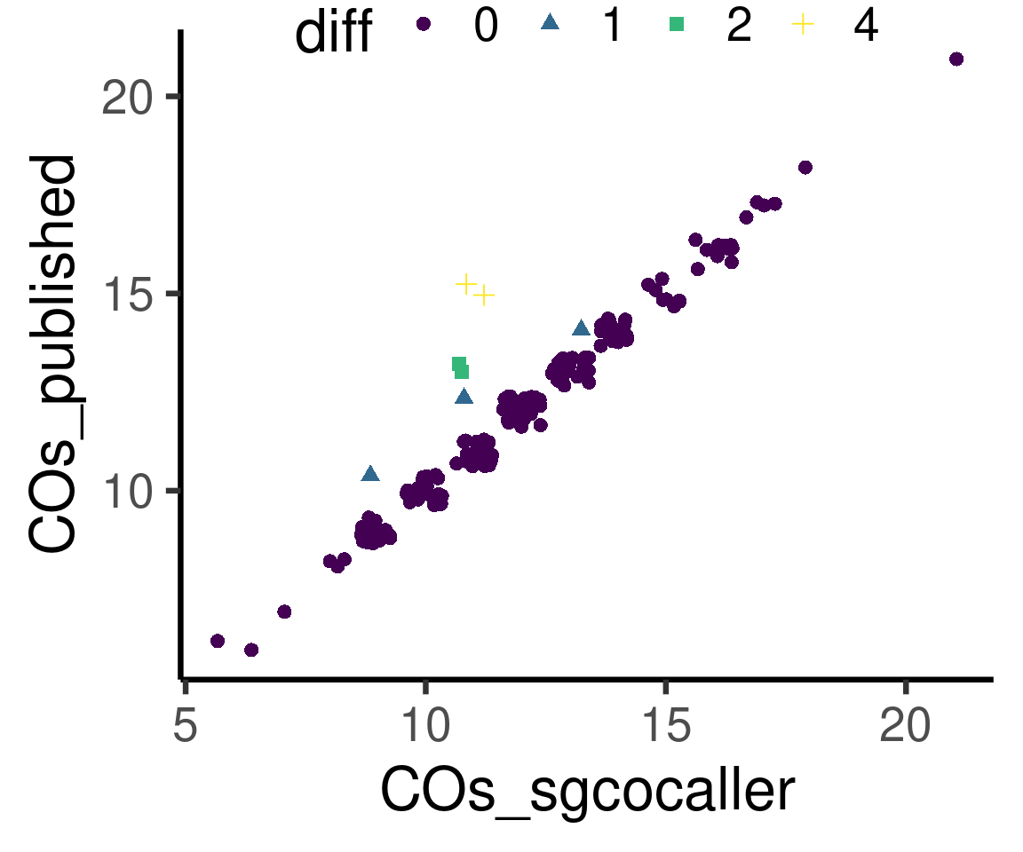
Differences in number of crossovers called by the two methods
| Version | Author | Date |
|---|---|---|
| 3883a5d | rlyu | 2022-01-10 |
# ggplot(data = hinch_cos,
#        mapping = aes(x = "Hinch Published",
#                      y = COs_hinch)) + geom_boxplot()+ geom_jitter()+
#   theme_classic()
#
# ggplot(data = hinch_cos,
#        mapping = aes( x = COs_hinch)) + geom_histogram(stat = "count")+
#   theme_classic()
# ggplot(data = sgcocaller_cos,
#        mapping = aes( x = COs_sgcocaller)) + geom_histogram(stat = "count")+
#   theme_classic()
The cells with discrepancy in number of crossovers called:
sgcocaller_cos %>% left_join(hinch_cos) %>% filter(COs_sgcocaller != COs_hinch)Joining, by = "SRR"# A tibble: 7 × 3
SRR COs_sgcocaller COs_hinch
<chr> <int> <int>
1 SRR8454715 11 15
2 SRR8454799 11 13
3 SRR8454804 11 13
4 SRR8454819 11 12
5 SRR8454825 11 15
6 SRR8454838 13 14
7 SRR8454863 9 10We can find the cell which has the largest difference in the number of crossovers called by the two methods:
sgcocaller_cos %>% left_join(hinch_cos) %>%
  mutate(diff = (COs_hinch - COs_sgcocaller)) %>%
  filter(diff>3)
Joining, by = "SRR"# A tibble: 2 × 4
SRR COs_sgcocaller COs_hinch diff
<chr> <int> <int> <int>
1 SRR8454715 11 15 4
2 SRR8454825 11 15 4We can then list the cells and chrs that have different number of crossovers called by the two methods for cell SRR8454715:
sgcocaller_cos <- called_co_df %>% group_by(SRR,chr) %>% summarise(ChrCOs_sgcocaller = n())`summarise()` has grouped output by 'SRR'. You can override using the `.groups` argument.hinch_cos <- pub_co %>% group_by(SRR,chr) %>% summarise(ChrCOs_hinch = n())`summarise()` has grouped output by 'SRR'. You can override using the `.groups` argument.hinch_cos %>% full_join(sgcocaller_cos) %>% filter(SRR == "SRR8454715")Joining, by = c("SRR", "chr")# A tibble: 11 × 4
# Groups: SRR [1]
SRR chr ChrCOs_hinch ChrCOs_sgcocaller
<chr> <chr> <int> <int>
1 SRR8454715 chr1 1 1
2 SRR8454715 chr10 1 1
3 SRR8454715 chr12 1 1
4 SRR8454715 chr18 2 NA
5 SRR8454715 chr19 1 1
6 SRR8454715 chr2 1 1
7 SRR8454715 chr3 1 1
8 SRR8454715 chr6 1 1
9 SRR8454715 chr7 3 1
10 SRR8454715 chr8 2 2
11 SRR8454715 chr9 1 1And then plot the alternative allele frequencies for the chromosomes that do not have the same number of crossovers called:
cell <- "SRR8454715"

SRR8454715_af <- getCellAFTrack(chrom = "chr7",
                                path_loc = dataset_dir,sampleName = "hinch",
                                barcodeFile = barcodeFile_path,
                                co_count = hinch_co_counts,
                                nwindow = 500,
                                chunk = 50000L,
                                cellBarcode = cell)
pub_co_range <- GRanges(seqnames = pub_co[pub_co$SRR==cell,]$chr,
IRanges(start = pub_co[pub_co$SRR==cell,]$crossover_breakpoint_leftpos,
end = pub_co[pub_co$SRR==cell,]$crossover_breakpoint_rightpos))Two extra crossovers on chromosome 17 were called from the original paper:
pub_co_chr7 <- AnnotationTrack(pub_co_range[seqnames(pub_co_range)=="chr7"],
                              name = "chr7 published CO ranges")
pub_co_chr7 <- setPar(pub_co_chr7,"background.title","lightblue")
Note that the behaviour of the 'setPar' method has changed. You need to reassign the result to an object for the side effects to happen. Pass-by-reference semantic is no longer supported.SRR8454715_af_ht <- HighlightTrack(trackList = list(gtrack, SRR8454715_af$af_track,
pub_co_chr7),
range = SRR8454715_af$co_range[seqnames(SRR8454715_af$co_range)=="chr7"])
plotTracks(SRR8454715_af_ht)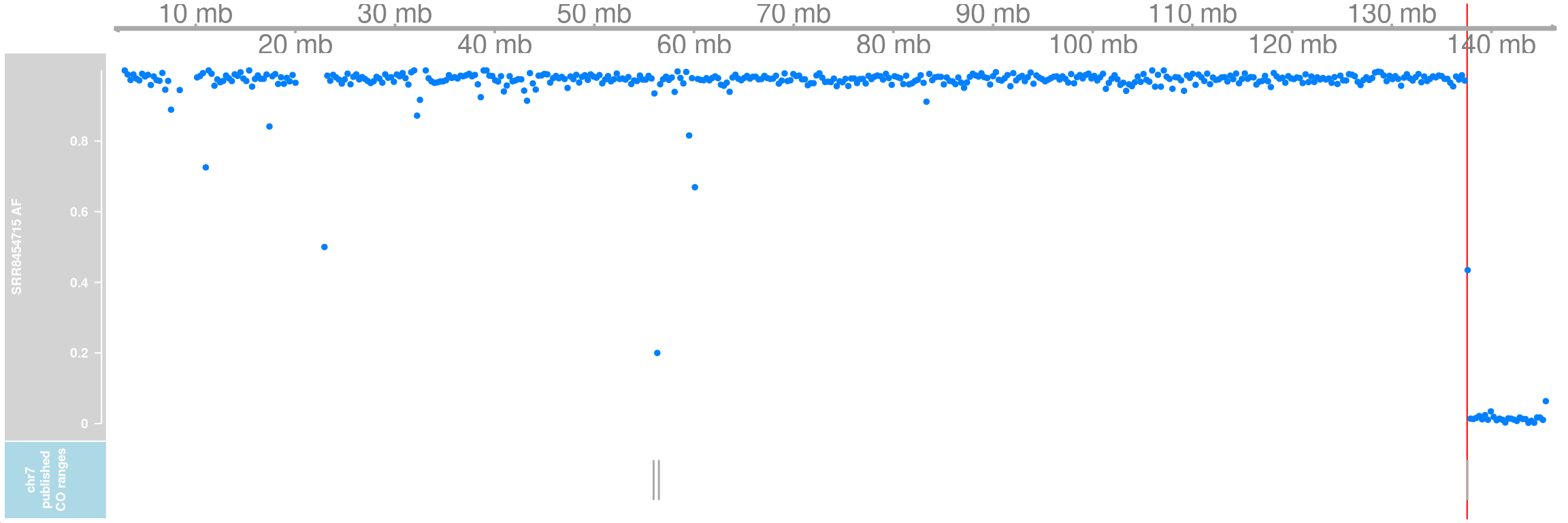
| Version | Author | Date |
|---|---|---|
| 3883a5d | rlyu | 2022-01-10 |
SRR8454715_af_chr18 <- getCellAFTrack(chrom = "chr18",
                                path_loc = dataset_dir,sampleName = "hinch",
                                barcodeFile = barcodeFile_path,
                                co_count = hinch_co_counts,
                                nwindow = 300,
                                chunk = 50000L,
                                cellBarcode = cell)
Two extra crossovers on chromosome 18 were called from the original paper:
pub_co_chr18 <- AnnotationTrack(pub_co_range[seqnames(pub_co_range)=="chr18"],
                                  name = "chr18 published CO ranges")
pub_co_chr18 <- setPar(pub_co_chr18,"background.title","lightblue")
Note that the behaviour of the 'setPar' method has changed. You need to reassign the result to an object for the side effects to happen. Pass-by-reference semantic is no longer supported.SRR8454715_af_ht <- HighlightTrack(trackList =
list(gtrack, SRR8454715_af_chr18$af_track,
pub_co_chr18),
range = SRR8454715_af_chr18$co_range[seqnames(SRR8454715_af_chr18$co_range)=="chr18"])
plotTracks(SRR8454715_af_ht)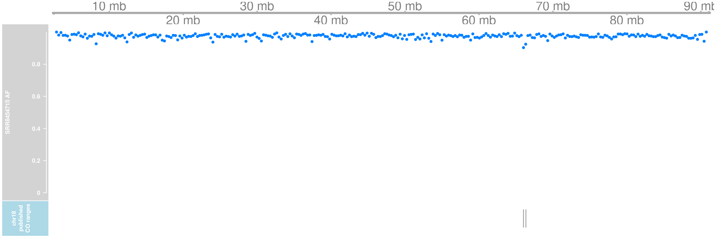
| Version | Author | Date |
|---|---|---|
| 3883a5d | rlyu | 2022-01-10 |
It is justifiable that comapr classify these 4 crossovers as false positives.
Summary
We have demonstrated the application of sgcocaller to find the haplotype states for the list of cell barcodes against the list of informative SNP markers using a binomial Hidden Markov Model. We have also showed the functionality of comapr for downstream analyses including cell quality control, finding crossover intervals, visualising crossover regions, calculating genetic distances and resampling testings for sample group comparisons. In addition, the tunable filtering parameters for calling crossovers enable comapr to be applied for datasets with different coverages.
Session info
sessionInfo()R version 4.1.0 (2021-05-18)
Platform: x86_64-pc-linux-gnu (64-bit)
Running under: Red Hat Enterprise Linux 8.4 (Ootpa)
Matrix products: default
BLAS/LAPACK: /usr/lib64/libopenblasp-r0.3.12.so
locale:
[1] LC_CTYPE=en_AU.UTF-8 LC_NUMERIC=C
[3] LC_TIME=en_AU.UTF-8 LC_COLLATE=en_AU.UTF-8
[5] LC_MONETARY=en_AU.UTF-8 LC_MESSAGES=en_AU.UTF-8
[7] LC_PAPER=en_AU.UTF-8 LC_NAME=C
[9] LC_ADDRESS=C LC_TELEPHONE=C
[11] LC_MEASUREMENT=en_AU.UTF-8 LC_IDENTIFICATION=C
attached base packages:
[1] grid parallel stats4 stats graphics grDevices utils
[8] datasets methods base
other attached packages:
[1] SummarizedExperiment_1.22.0 Biobase_2.52.0
[3] MatrixGenerics_1.4.3 matrixStats_0.61.0
[5] BiocParallel_1.26.2 Gviz_1.36.2
[7] GenomicRanges_1.44.0 GenomeInfoDb_1.28.4
[9] IRanges_2.26.0 S4Vectors_0.30.1
[11] BiocGenerics_0.38.0 dplyr_1.0.7
[13] ggplot2_3.3.5 comapr_0.99.37
loaded via a namespace (and not attached):
[1] backports_1.2.1 circlize_0.4.13 Hmisc_4.5-0
[4] workflowr_1.6.2 BiocFileCache_2.0.0 plyr_1.8.6
[7] lazyeval_0.2.2 splines_4.1.0 digest_0.6.28
[10] foreach_1.5.1 ensembldb_2.16.4 htmltools_0.5.2
[13] fansi_0.5.0 magrittr_2.0.1 checkmate_2.0.0
[16] memoise_2.0.0 BSgenome_1.60.0 cluster_2.1.2
[19] Biostrings_2.60.2 prettyunits_1.1.1 jpeg_0.1-9
[22] colorspace_2.0-2 blob_1.2.2 rappdirs_0.3.3
[25] xfun_0.26 crayon_1.4.1 RCurl_1.98-1.5
[28] jsonlite_1.7.2 survival_3.2-11 VariantAnnotation_1.38.0
[31] iterators_1.0.13 glue_1.4.2 gtable_0.3.0
[34] zlibbioc_1.38.0 XVector_0.32.0 DelayedArray_0.18.0
[37] shape_1.4.6 scales_1.1.1 DBI_1.1.1
[40] Rcpp_1.0.7 viridisLite_0.4.0 progress_1.2.2
[43] htmlTable_2.2.1 foreign_0.8-81 bit_4.0.4
[46] Formula_1.2-4 htmlwidgets_1.5.4 httr_1.4.2
[49] RColorBrewer_1.1-2 ellipsis_0.3.2 pkgconfig_2.0.3
[52] XML_3.99-0.8 farver_2.1.0 nnet_7.3-16
[55] dbplyr_2.1.1 utf8_1.2.2 labeling_0.4.2
[58] tidyselect_1.1.1 rlang_0.4.11 reshape2_1.4.4
[61] later_1.3.0 AnnotationDbi_1.54.1 munsell_0.5.0
[64] tools_4.1.0 cachem_1.0.6 cli_3.0.1
[67] generics_0.1.0 RSQLite_2.2.8 evaluate_0.14
[70] stringr_1.4.0 fastmap_1.1.0 yaml_2.2.1
[73] knitr_1.36 bit64_4.0.5 fs_1.5.0
[76] purrr_0.3.4 KEGGREST_1.32.0 AnnotationFilter_1.16.0
[79] whisker_0.4 xml2_1.3.2 biomaRt_2.48.3
[82] compiler_4.1.0 rstudioapi_0.13 plotly_4.9.4.1
[85] filelock_1.0.2 curl_4.3.2 png_0.1-7
[88] statmod_1.4.36 tibble_3.1.4 stringi_1.7.4
[91] highr_0.9 GenomicFeatures_1.44.2 lattice_0.20-44
[94] ProtGenerics_1.24.0 Matrix_1.3-3 vctrs_0.3.8
[97] pillar_1.6.3 lifecycle_1.0.1 jquerylib_0.1.4
[100] GlobalOptions_0.1.2 data.table_1.14.2 bitops_1.0-7
[103] httpuv_1.6.3 rtracklayer_1.52.1 R6_2.5.1
[106] BiocIO_1.2.0 latticeExtra_0.6-29 promises_1.2.0.1
[109] gridExtra_2.3 codetools_0.2-18 dichromat_2.0-0
[112] assertthat_0.2.1 rprojroot_2.0.2 rjson_0.2.20
[115] withr_2.4.2 GenomicAlignments_1.28.0 Rsamtools_2.8.0
[118] GenomeInfoDbData_1.2.6 hms_1.1.1 rpart_4.1-15
[121] tidyr_1.1.4 rmarkdown_2.11 git2r_0.28.0
[124] biovizBase_1.40.0 base64enc_0.1-3 restfulr_0.0.13 References
devtools::session_info()─ Session info ───────────────────────────────────────────────────────────────
setting value
version R version 4.1.0 (2021-05-18)
os Red Hat Enterprise Linux 8.4 (Ootpa)
system x86_64, linux-gnu
ui X11
language (EN)
collate en_AU.UTF-8
ctype en_AU.UTF-8
tz Australia/Melbourne
date 2022-01-20
─ Packages ───────────────────────────────────────────────────────────────────
package * version date lib source
AnnotationDbi 1.54.1 2021-06-08 [1] Bioconductor
AnnotationFilter 1.16.0 2021-05-19 [1] Bioconductor
assertthat 0.2.1 2019-03-21 [1] CRAN (R 4.1.0)
backports 1.2.1 2020-12-09 [1] CRAN (R 4.1.0)
base64enc 0.1-3 2015-07-28 [1] CRAN (R 4.1.0)
Biobase * 2.52.0 2021-05-19 [1] Bioconductor
BiocFileCache 2.0.0 2021-05-19 [1] Bioconductor
BiocGenerics * 0.38.0 2021-05-19 [1] Bioconductor
BiocIO 1.2.0 2021-05-19 [1] Bioconductor
BiocParallel * 1.26.2 2021-08-22 [1] Bioconductor
biomaRt 2.48.3 2021-08-15 [1] Bioconductor
Biostrings 2.60.2 2021-08-05 [1] Bioconductor
biovizBase 1.40.0 2021-05-19 [1] Bioconductor
bit 4.0.4 2020-08-04 [1] CRAN (R 4.1.0)
bit64 4.0.5 2020-08-30 [1] CRAN (R 4.1.0)
bitops 1.0-7 2021-04-24 [1] CRAN (R 4.1.0)
blob 1.2.2 2021-07-23 [1] CRAN (R 4.1.0)
BSgenome 1.60.0 2021-05-19 [1] Bioconductor
cachem 1.0.6 2021-08-19 [1] CRAN (R 4.1.0)
callr 3.7.0 2021-04-20 [1] CRAN (R 4.1.0)
checkmate 2.0.0 2020-02-06 [1] CRAN (R 4.1.0)
circlize 0.4.13 2021-06-09 [1] CRAN (R 4.1.0)
cli 3.0.1 2021-07-17 [1] CRAN (R 4.1.0)
cluster 2.1.2 2021-04-17 [2] CRAN (R 4.1.0)
codetools 0.2-18 2020-11-04 [2] CRAN (R 4.1.0)
colorspace 2.0-2 2021-06-24 [1] CRAN (R 4.1.0)
comapr * 0.99.37 2021-11-28 [1] Github (ruqianl/comapr@aad1b6a)
crayon 1.4.1 2021-02-08 [1] CRAN (R 4.1.0)
curl 4.3.2 2021-06-23 [1] CRAN (R 4.1.0)
data.table 1.14.2 2021-09-27 [1] CRAN (R 4.1.0)
DBI 1.1.1 2021-01-15 [1] CRAN (R 4.1.0)
dbplyr 2.1.1 2021-04-06 [1] CRAN (R 4.1.0)
DelayedArray 0.18.0 2021-05-19 [1] Bioconductor
desc 1.4.0 2021-09-28 [1] CRAN (R 4.1.0)
devtools 2.4.2 2021-06-07 [1] CRAN (R 4.1.0)
dichromat 2.0-0 2013-01-24 [1] CRAN (R 4.1.0)
digest 0.6.28 2021-09-23 [1] CRAN (R 4.1.0)
dplyr * 1.0.7 2021-06-18 [1] CRAN (R 4.1.0)
ellipsis 0.3.2 2021-04-29 [1] CRAN (R 4.1.0)
ensembldb 2.16.4 2021-08-05 [1] Bioconductor
evaluate 0.14 2019-05-28 [1] CRAN (R 4.1.0)
fansi 0.5.0 2021-05-25 [1] CRAN (R 4.1.0)
farver 2.1.0 2021-02-28 [1] CRAN (R 4.1.0)
fastmap 1.1.0 2021-01-25 [1] CRAN (R 4.1.0)
filelock 1.0.2 2018-10-05 [1] CRAN (R 4.1.0)
foreach 1.5.1 2020-10-15 [1] CRAN (R 4.1.0)
foreign 0.8-81 2020-12-22 [2] CRAN (R 4.1.0)
Formula 1.2-4 2020-10-16 [1] CRAN (R 4.1.0)
fs 1.5.0 2020-07-31 [1] CRAN (R 4.1.0)
generics 0.1.0 2020-10-31 [1] CRAN (R 4.1.0)
GenomeInfoDb * 1.28.4 2021-09-05 [1] Bioconductor
GenomeInfoDbData 1.2.6 2021-09-30 [1] Bioconductor
GenomicAlignments 1.28.0 2021-05-19 [1] Bioconductor
GenomicFeatures 1.44.2 2021-08-26 [1] Bioconductor
GenomicRanges * 1.44.0 2021-05-19 [1] Bioconductor
ggplot2 * 3.3.5 2021-06-25 [1] CRAN (R 4.1.0)
git2r 0.28.0 2021-01-10 [1] CRAN (R 4.1.0)
GlobalOptions 0.1.2 2020-06-10 [1] CRAN (R 4.1.0)
glue 1.4.2 2020-08-27 [1] CRAN (R 4.1.0)
gridExtra 2.3 2017-09-09 [1] CRAN (R 4.1.0)
gtable 0.3.0 2019-03-25 [1] CRAN (R 4.1.0)
Gviz * 1.36.2 2021-07-04 [1] Bioconductor
highr 0.9 2021-04-16 [1] CRAN (R 4.1.0)
Hmisc 4.5-0 2021-02-28 [1] CRAN (R 4.1.0)
hms 1.1.1 2021-09-26 [1] CRAN (R 4.1.0)
htmlTable 2.2.1 2021-05-18 [1] CRAN (R 4.1.0)
htmltools 0.5.2 2021-08-25 [1] CRAN (R 4.1.0)
htmlwidgets 1.5.4 2021-09-08 [1] CRAN (R 4.1.0)
httpuv 1.6.3 2021-09-09 [1] CRAN (R 4.1.0)
httr 1.4.2 2020-07-20 [1] CRAN (R 4.1.0)
IRanges * 2.26.0 2021-05-19 [1] Bioconductor
iterators 1.0.13 2020-10-15 [1] CRAN (R 4.1.0)
jpeg 0.1-9 2021-07-24 [1] CRAN (R 4.1.0)
jquerylib 0.1.4 2021-04-26 [1] CRAN (R 4.1.0)
jsonlite 1.7.2 2020-12-09 [1] CRAN (R 4.1.0)
KEGGREST 1.32.0 2021-05-19 [1] Bioconductor
knitr 1.36 2021-09-29 [1] CRAN (R 4.1.0)
labeling 0.4.2 2020-10-20 [1] CRAN (R 4.1.0)
later 1.3.0 2021-08-18 [1] CRAN (R 4.1.0)
lattice 0.20-44 2021-05-02 [2] CRAN (R 4.1.0)
latticeExtra 0.6-29 2019-12-19 [1] CRAN (R 4.1.0)
lazyeval 0.2.2 2019-03-15 [1] CRAN (R 4.1.0)
lifecycle 1.0.1 2021-09-24 [1] CRAN (R 4.1.0)
magrittr 2.0.1 2020-11-17 [1] CRAN (R 4.1.0)
Matrix 1.3-3 2021-05-04 [2] CRAN (R 4.1.0)
MatrixGenerics * 1.4.3 2021-08-26 [1] Bioconductor
matrixStats * 0.61.0 2021-09-17 [1] CRAN (R 4.1.0)
memoise 2.0.0 2021-01-26 [1] CRAN (R 4.1.0)
munsell 0.5.0 2018-06-12 [1] CRAN (R 4.1.0)
nnet 7.3-16 2021-05-03 [2] CRAN (R 4.1.0)
pillar 1.6.3 2021-09-26 [1] CRAN (R 4.1.0)
pkgbuild 1.2.0 2020-12-15 [1] CRAN (R 4.1.0)
pkgconfig 2.0.3 2019-09-22 [1] CRAN (R 4.1.0)
pkgload 1.2.2 2021-09-11 [1] CRAN (R 4.1.0)
plotly 4.9.4.1 2021-06-18 [1] CRAN (R 4.1.0)
plyr 1.8.6 2020-03-03 [1] CRAN (R 4.1.0)
png 0.1-7 2013-12-03 [1] CRAN (R 4.1.0)
prettyunits 1.1.1 2020-01-24 [1] CRAN (R 4.1.0)
processx 3.5.2 2021-04-30 [1] CRAN (R 4.1.0)
progress 1.2.2 2019-05-16 [1] CRAN (R 4.1.0)
promises 1.2.0.1 2021-02-11 [1] CRAN (R 4.1.0)
ProtGenerics 1.24.0 2021-05-19 [1] Bioconductor
ps 1.6.0 2021-02-28 [1] CRAN (R 4.1.0)
purrr 0.3.4 2020-04-17 [1] CRAN (R 4.1.0)
R6 2.5.1 2021-08-19 [1] CRAN (R 4.1.0)
rappdirs 0.3.3 2021-01-31 [1] CRAN (R 4.1.0)
RColorBrewer 1.1-2 2014-12-07 [1] CRAN (R 4.1.0)
Rcpp 1.0.7 2021-07-07 [1] CRAN (R 4.1.0)
RCurl 1.98-1.5 2021-09-17 [1] CRAN (R 4.1.0)
remotes 2.4.1 2021-09-29 [1] CRAN (R 4.1.0)
reshape2 1.4.4 2020-04-09 [1] CRAN (R 4.1.0)
restfulr 0.0.13 2017-08-06 [1] CRAN (R 4.1.0)
rjson 0.2.20 2018-06-08 [1] CRAN (R 4.1.0)
rlang 0.4.11 2021-04-30 [1] CRAN (R 4.1.0)
rmarkdown 2.11 2021-09-14 [1] CRAN (R 4.1.0)
rpart 4.1-15 2019-04-12 [2] CRAN (R 4.1.0)
rprojroot 2.0.2 2020-11-15 [1] CRAN (R 4.1.0)
Rsamtools 2.8.0 2021-05-19 [1] Bioconductor
RSQLite 2.2.8 2021-08-21 [1] CRAN (R 4.1.0)
rstudioapi 0.13 2020-11-12 [1] CRAN (R 4.1.0)
rtracklayer 1.52.1 2021-08-15 [1] Bioconductor
S4Vectors * 0.30.1 2021-09-26 [1] Bioconductor
scales 1.1.1 2020-05-11 [1] CRAN (R 4.1.0)
sessioninfo 1.1.1 2018-11-05 [1] CRAN (R 4.1.0)
shape 1.4.6 2021-05-19 [1] CRAN (R 4.1.0)
statmod 1.4.36 2021-05-10 [1] CRAN (R 4.1.0)
stringi 1.7.4 2021-08-25 [1] CRAN (R 4.1.0)
stringr 1.4.0 2019-02-10 [1] CRAN (R 4.1.0)
SummarizedExperiment * 1.22.0 2021-05-19 [1] Bioconductor
survival 3.2-11 2021-04-26 [2] CRAN (R 4.1.0)
testthat 3.0.4 2021-07-01 [1] CRAN (R 4.1.0)
tibble 3.1.4 2021-08-25 [1] CRAN (R 4.1.0)
tidyr 1.1.4 2021-09-27 [1] CRAN (R 4.1.0)
tidyselect 1.1.1 2021-04-30 [1] CRAN (R 4.1.0)
usethis 2.0.1 2021-02-10 [1] CRAN (R 4.1.0)
utf8 1.2.2 2021-07-24 [1] CRAN (R 4.1.0)
VariantAnnotation 1.38.0 2021-05-19 [1] Bioconductor
vctrs 0.3.8 2021-04-29 [1] CRAN (R 4.1.0)
viridisLite 0.4.0 2021-04-13 [1] CRAN (R 4.1.0)
whisker 0.4 2019-08-28 [1] CRAN (R 4.1.0)
withr 2.4.2 2021-04-18 [1] CRAN (R 4.1.0)
workflowr 1.6.2 2020-04-30 [1] CRAN (R 4.1.0)
xfun 0.26 2021-09-14 [1] CRAN (R 4.1.0)
XML 3.99-0.8 2021-09-17 [1] CRAN (R 4.1.0)
xml2 1.3.2 2020-04-23 [1] CRAN (R 4.1.0)
XVector 0.32.0 2021-05-19 [1] Bioconductor
yaml 2.2.1 2020-02-01 [1] CRAN (R 4.1.0)
zlibbioc 1.38.0 2021-05-19 [1] Bioconductor
[1] /mnt/beegfs/mccarthy/scratch/general/rlyu/Software/R/Rlib/4.1.0/yeln
[2] /opt/R/4.1.0/lib/R/library