Method concordance

workflowr

• Summary
• Checks
• Past versions

Last updated: 2024-01-01

Checks: 7 0

Knit directory: mage_2020_marker-gene-benchmarking/

This reproducible R Markdown analysis was created with workflowr (version 1.7.0). The Checks tab describes the reproducibility checks that were applied when the results were created. The Past versions tab lists the development history.

---

R Markdown file: up-to-date

Great! Since the R Markdown file has been committed to the Git repository, you know the exact version of the code that produced these results.

Environment: empty

Great job! The global environment was empty. Objects defined in the global environment can affect the analysis in your R Markdown file in unknown ways. For reproduciblity it’s best to always run the code in an empty environment.

Seed: set.seed(20190102)

The command set.seed(20190102) was run prior to running the code in the R Markdown file. Setting a seed ensures that any results that rely on randomness, e.g. subsampling or permutations, are reproducible.

Session information: recorded

Great job! Recording the operating system, R version, and package versions is critical for reproducibility.

Cache: none

Nice! There were no cached chunks for this analysis, so you can be confident that you successfully produced the results during this run.

File paths: relative

Great job! Using relative paths to the files within your workflowr project makes it easier to run your code on other machines.

Repository version: 2632193

Great! You are using Git for version control. Tracking code development and connecting the code version to the results is critical for reproducibility.

The results in this page were generated with repository version 2632193. See the Past versions tab to see a history of the changes made to the R Markdown and HTML files.

Note that you need to be careful to ensure that all relevant files for the analysis have been committed to Git prior to generating the results (you can use wflow_publish or wflow_git_commit). workflowr only checks the R Markdown file, but you know if there are other scripts or data files that it depends on. Below is the status of the Git repository when the results were generated:

Ignored files:
    Ignored:    .Renviron
    Ignored:    .Rhistory
    Ignored:    .Rproj.user/
    Ignored:    .snakemake/
    Ignored:    NSForest/.Rhistory
    Ignored:    NSForest/NS-Forest_v3_Extended_Binary_Markers_Supplmental.csv
    Ignored:    NSForest/NS-Forest_v3_Full_Results.csv
    Ignored:    NSForest/NSForest3_medianValues.csv
    Ignored:    NSForest/NSForest_v3_Final_Result.csv
    Ignored:    NSForest/__pycache__/
    Ignored:    NSForest/data/
    Ignored:    RankCorr/picturedRocks/__pycache__/
    Ignored:    benchmarks/
    Ignored:    config/
    Ignored:    data/cellmarker/
    Ignored:    data/downloaded_data/
    Ignored:    data/expert_annotations/
    Ignored:    data/expert_mgs/
    Ignored:    data/raw_data/
    Ignored:    data/real_data/
    Ignored:    data/sim_data/
    Ignored:    data/sim_mgs/
    Ignored:    data/special_real_data/
    Ignored:    figures/
    Ignored:    logs/
    Ignored:    results/
    Ignored:    weights/

Unstaged changes:
    Deleted:    analysis/expert-mgs-direction.Rmd
    Modified:   smash-fork

Note that any generated files, e.g. HTML, png, CSS, etc., are not included in this status report because it is ok for generated content to have uncommitted changes.

---

These are the previous versions of the repository in which changes were made to the R Markdown (analysis/concordance.Rmd) and HTML (public/concordance.html) files. If you’ve configured a remote Git repository (see ?wflow_git_remote), click on the hyperlinks in the table below to view the files as they were in that past version.

File	Version	Author	Date	Message
Rmd	2632193	Jeffrey Pullin	2024-01-01	Implement revisions
Rmd	bc98f8b	Jeffrey Pullin	2023-11-20	GB resubmission July 2023
Rmd	f54229a	Jeffrey Pullin	2023-06-17	Draft additional concordance analysis
html	fcecf65	Jeffrey Pullin	2022-09-09	Build site.
Rmd	0c2eafc	Jeffrey Pullin	2022-09-09	Update website
html	af96b34	Jeffrey Pullin	2022-08-30	Build site.
Rmd	854d178	Jeffrey Pullin	2022-07-21	Update concordance analysis
html	0e47874	Jeffrey Pullin	2022-05-04	Build site.
html	b5045c1	Jeffrey Pullin	2022-05-02	Build site.
Rmd	048156f	Jeffrey Pullin	2022-05-02	Tweak analysis outputs
html	048156f	Jeffrey Pullin	2022-05-02	Tweak analysis outputs
html	8b989e1	Jeffrey Pullin	2022-05-02	Build site.
html	0548273	Jeffrey Pullin	2022-05-02	Build site.
Rmd	50bca7c	Jeffrey Pullin	2022-05-02	workflowr::wflow_publish(all = TRUE, republish = TRUE)
html	50bca7c	Jeffrey Pullin	2022-05-02	workflowr::wflow_publish(all = TRUE, republish = TRUE)
html	5cc008f	Jeffrey Pullin	2022-02-09	Build site.
Rmd	d1aca16	Jeffrey Pullin	2022-02-09	Refresh website
html	d1aca16	Jeffrey Pullin	2022-02-09	Refresh website
Rmd	aca9ad2	Jeffrey Pullin	2021-11-29	Various changes made in the last days before thesis submission
Rmd	d3804d1	Jeffrey Pullin	2021-09-23	Polish analyses
Rmd	b520587	Jeffrey Pullin	2021-09-21	Polish concordance analysis
Rmd	211b2f6	Jeffrey Pullin	2021-09-21	Add ranking plots concordance analysis
Rmd	92d3bf0	Jeffrey Pullin	2021-08-02	Add code to create plots for ECSSC talk
html	61ee246	Jeffrey Pullin	2021-04-13	Build site.
Rmd	b5b2a88	Jeffrey Pullin	2021-04-13	Add new results
Rmd	b895f6e	Jeffrey Pullin	2021-04-05	Add cluster analysis
Rmd	d036935	Jeffrey Pullin	2021-03-31	Refactor concordance analysis
html	ca82ce0	Jeffrey Pullin	2021-02-16	Build site.
html	2863555	Jeffrey Pullin	2021-02-10	Build site.
Rmd	1ad9d6d	Jeffrey Pullin	2021-02-10	Add workflowr website

---

library(tibble)
library(dplyr)
library(ggupset)
library(ggplot2)
library(tidyr)
library(SingleCellExperiment)
library(logisticPCA)
library(pals)
library(topconfects)
library(patchwork)
library(ggrepel)
library(purrr)
library(scater)
library(forcats)
library(ggdendro)

source(here::here("code", "top-genes.R"))
source(here::here("code", "analysis-utils.R"))
source(here::here("code", "plot-utils.R"))

#' Get the top marker genes for a specific cluster
#' 
#' @param output The output of a (data, method) pair run
#' @param cluster The cluster to extract marker genes for
#' @param n The number of marker genes to extract
#' 
#' @return A vector of gene names
#' 
get_top_marker_genes <- function(output, cluster, n) {
  result <- output$result
  result <- result[result$cluster == cluster, ]
  result <- get_top_sel_mgs(result, n = n)
  mgs <- result$gene
  mgs
}

concordance_data <- retrieve_real_data_parameters() %>% 
  filter(!(data_id %in% c("citeseq", "mesenchymal", "ss3_pbmc", "zhao"))) %>% 
  rowwise() %>% 
  mutate(mgs = list(readRDS(full_filename)$result)) %>%
  mutate(mgs = list(split(mgs, mgs$cluster))) %>% 
  ungroup() %>% 
  unnest(cols = mgs) %>% 
  rowwise() %>% 
  mutate(cluster = mgs$cluster[[1]]) %>% 
  ungroup()
 
poor_methods <- c("random", "binom", "difference", "lm")

long_data <- concordance_data %>%
  filter(!(method %in% poor_methods)) %>% 
  filter(data_id == "pbmc3k", cluster == "B") %>% 
  rowwise() %>% 
  mutate(mgs = list(get_top_sel_mgs(mgs, n = 100)$gene)) %>% 
  ungroup() %>% 
  unnest_longer(col = mgs) %>% 
  # Not sure why this occurs.
  filter(!is.na(mgs))

binary_data <- model.matrix(~ 0 + . , data = long_data["mgs"])

cluster_data <- cbind(
  pars = long_data$pars, 
  as.data.frame(binary_data)
) %>% 
  group_by(pars) %>% 
  summarise(across(everything(), sum))

cluster_mat <- as.matrix(cluster_data[, -1])

Dimensionality reduction: PCA

pca <- prcomp(cluster_mat)
pca_plot <- tibble(
  pc1 = pca$x[, 1], 
  pc2 = pca$x[, 2], 
  pars = cluster_data$pars,
  plot_pars = pars_lookup[cluster_data$pars]
) %>% 
  rowwise() %>% 
  mutate(method = strsplit(pars, "[_]")[[1]][1]) %>%
  ungroup() %>% 
  ggplot(aes(x = pc1, y = pc2, label = plot_pars, colour = method)) + 
  geom_point(size = 3) + 
  geom_text_repel(
    aes(label = plot_pars), 
    colour = "black", 
    max.overlaps = 20) + 
  labs(
    x = "Principal component 1", 
    y = "Principal component 2",
    colour = "Package"
  ) + 
  theme_bw()
pca_plot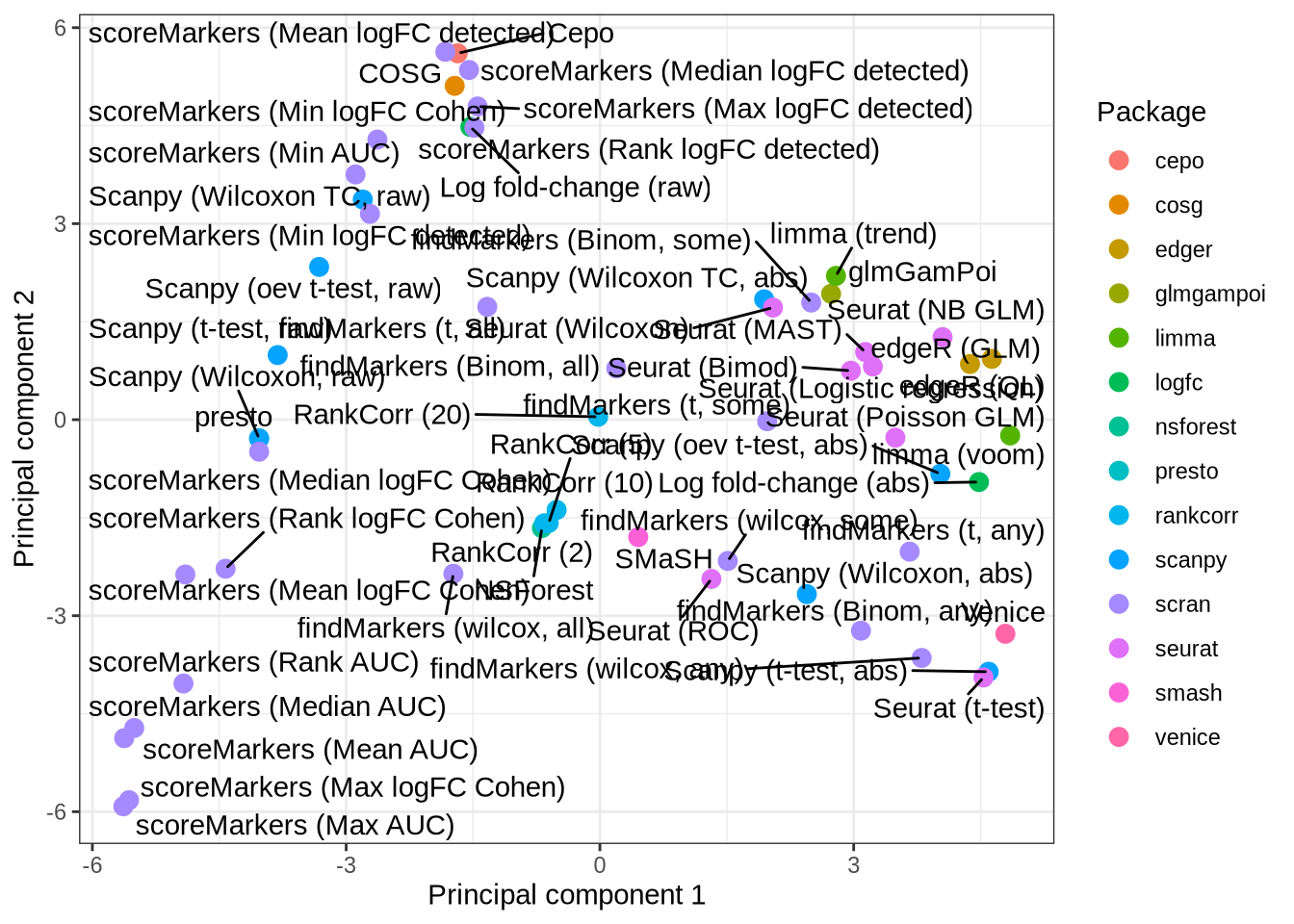

saveRDS(
  pca_plot, 
  here::here("figures", "raw", "concordance-pca-plot-with-text.rds")
)

Intersection dendrogram

n <- 10
all_concordance_data <- concordance_data %>% 
  rowwise() %>% 
  mutate(mgs = list(get_top_sel_mgs(mgs, n = n)$gene)) %>% 
  ungroup() %>% 
  select(pars, method, cluster, data_id, mgs)

intersection_data <- all_concordance_data %>% 
  expand_grid(pars_2 = unique(all_concordance_data$pars)) %>% 
  left_join(
    dplyr::rename(all_concordance_data, mgs_2 = mgs), 
    by = c("pars_2" = "pars", "cluster")
  ) %>% 
  rowwise() %>% 
  mutate(prop_intersect = length(intersect(mgs, mgs_2)) / n) %>% 
  ungroup() %>% 
  select(pars, pars_2, cluster, prop_intersect)  %>%
  group_by(pars, pars_2) %>% 
  summarise(prop_intersect = mean(prop_intersect), .groups = "drop") %>% 
  pivot_wider(names_from = pars, values_from = prop_intersect)

intersection_mat <- as.matrix(intersection_data[, -1])
rownames(intersection_mat) <- intersection_data[[1]]

hier_clust <- hclust(dist(intersection_mat))
hier_clust$labels <- pars_lookup[hier_clust$labels]

hier_clust_data <- dendro_data(hier_clust, type = "rectangle")

dendrogram_plot <- ggplot() +
  geom_segment(data = segment(hier_clust_data), 
               aes(x = x, y = y, xend = xend, yend = yend)
  ) +
  geom_text(data = label(hier_clust_data), 
            aes(x = x, y = y, label = label, hjust = 0), 
            size = 4
  ) +
  coord_flip(xlim = c(3, 57)) +
  scale_y_reverse(limits = c(4, -1.5)) + 
  theme_dendro()
dendrogram_plot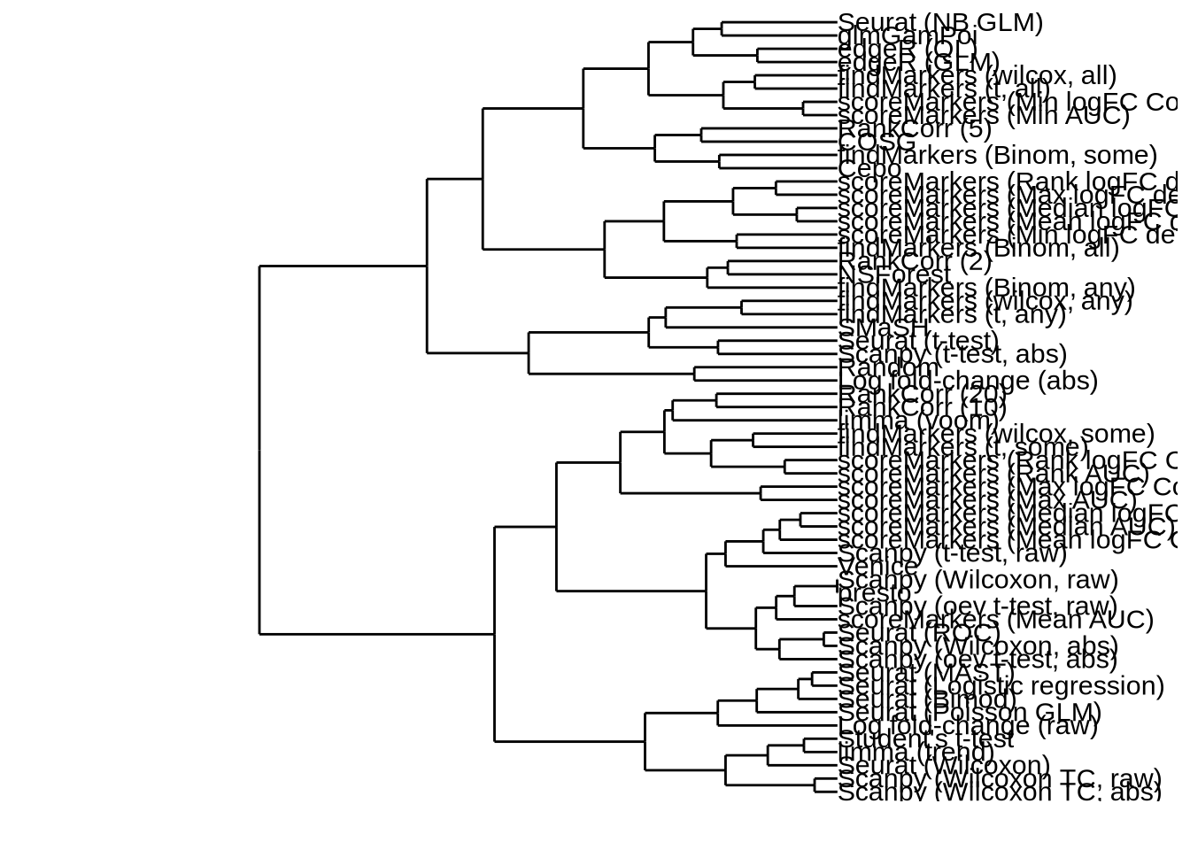

saveRDS(dendrogram_plot, here::here("figures", "raw", "dendrogram.rds"))

raw_pars <- c("scanpy_tover_rankby_raw", "scanpy_wilcoxon_rankby_raw", "presto",
              "logfc_raw", "scanpy_t_rankby_raw",
              "scanpy_wilcoxontiecorrect_rankby_raw")
non_rank_pars <- c("rankcorr_2", "rankcorr_10", "rankcorr_20", "rankcorr_5", 
                   "nsforest")

dendro_info_data <- tibble(
  pars = rownames(hier_clust_data$labels),
) %>% 
  mutate(plot_pars = pars_lookup[pars]) %>% 
  mutate(plot_pars = factor(plot_pars, levels = hier_clust_data$labels$label)) %>% 
  mutate(
    is_raw = as.character(pars %in% raw_pars),
    is_non_rank = as.character(pars %in% non_rank_pars)
  ) %>% 
  left_join(
    select(concordance_data, c(pars, method)), 
    by = "pars"
  ) %>% 
  mutate(plot_method = method_lookup[method]) %>% 
  pivot_longer(cols = c(is_raw, is_non_rank, plot_method), 
               names_to = "criteria")

is_raw_plot <- dendro_info_data %>% 
  filter(criteria == "is_raw") %>% 
  mutate(Direction = value) %>% 
  mutate(Direction = if_else(Direction == "FALSE", 
                             "Either", "Up-regulated only")) %>% 
  mutate(Direction = factor(Direction, levels = c("Up-regulated only", "Either"))) %>% 
  ggplot(aes(x = criteria, y = plot_pars)) + 
  geom_tile(aes(fill = Direction), colour = "black")  +
  scale_fill_manual(values = c("#E41A1C", "#377EB8")) + 
  theme_bw() + 
  theme(
    panel.grid.major = element_blank(),
    panel.grid.minor = element_blank(),
    panel.border = element_blank(),
    axis.text = element_blank(), 
    axis.ticks = element_blank(), 
    axis.title = element_blank()
  )
is_raw_plot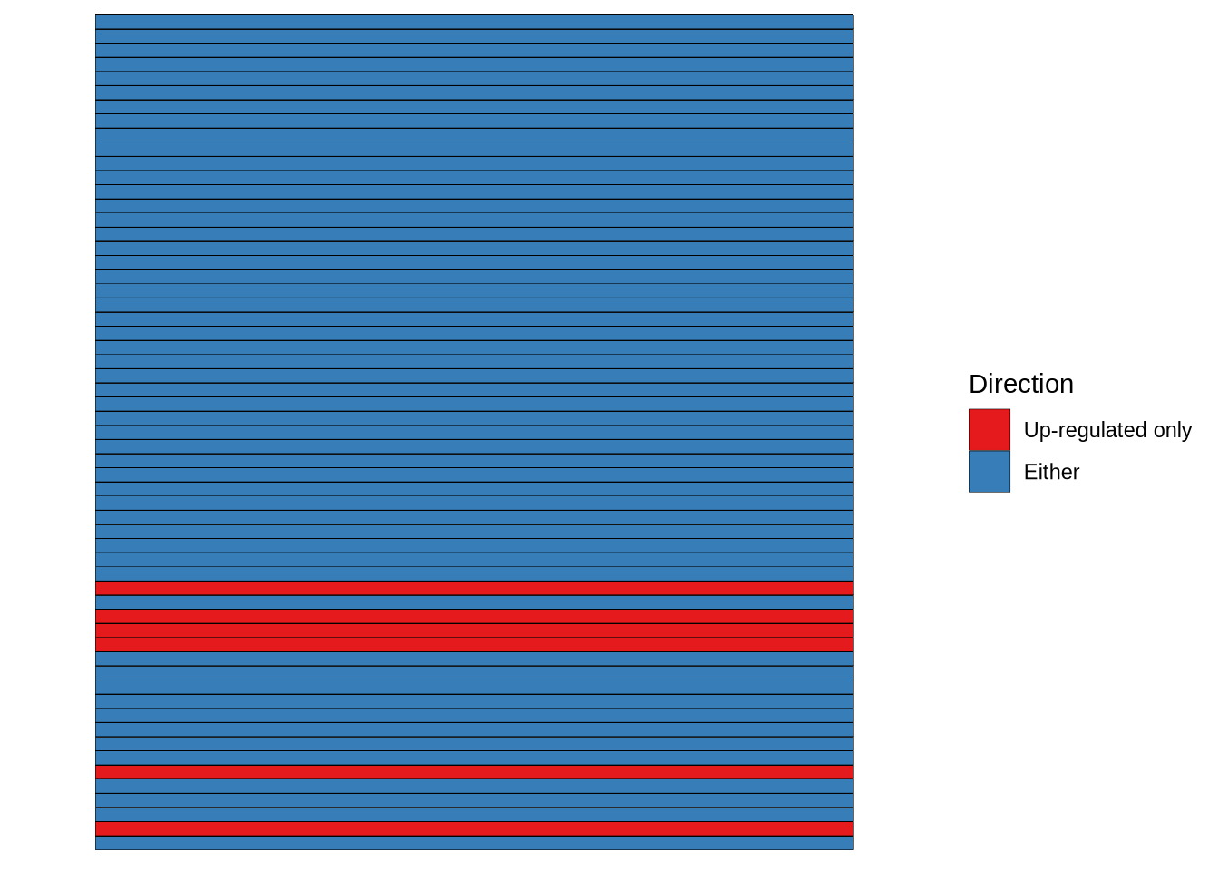

is_non_rank_plot <- dendro_info_data %>% 
  filter(criteria == "is_non_rank") %>% 
  mutate(Strategy = if_else(value == "FALSE", 
                             "Ranking", "Fixed set")) %>% 
  mutate(`Rank or set` = factor(Strategy, levels = c("Fixed set", "Ranking"))) %>% 
  ggplot(aes(x = criteria, y = plot_pars)) + 
  geom_tile(aes(fill = `Rank or set`), colour = "black")  +
  scale_fill_manual(values = c("#66C2A5", "#FC8D62")) + 
  theme_bw() + 
  theme(
    panel.grid.major = element_blank(),
    panel.grid.minor = element_blank(),
    panel.border = element_blank(),
    axis.text = element_blank(), 
    axis.ticks = element_blank(), 
    axis.title = element_blank()
  )
is_non_rank_plot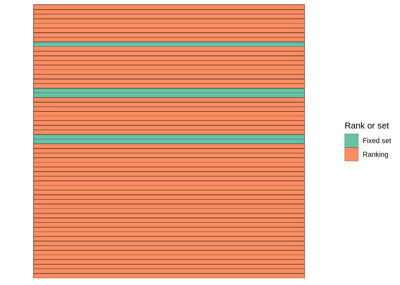

package_plot <- dendro_info_data %>% 
  filter(criteria == "plot_method") %>% 
  mutate(Package = value) %>% 
  ggplot(aes(x = criteria, y = plot_pars)) + 
  geom_tile(aes(fill = Package), colour = "black")  +
  package_fill + 
  theme_bw() + 
  theme(
    panel.grid.major = element_blank(),
    panel.grid.minor = element_blank(),
    panel.border = element_blank(),
    axis.text = element_blank(), 
    axis.ticks = element_blank(), 
    axis.title = element_blank()
  )
package_plot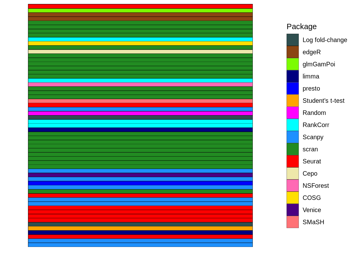

saveRDS(is_raw_plot, here::here("figures", "raw", "raw-info.rds"))
saveRDS(is_non_rank_plot, here::here("figures", "raw", "strategy-info.rds"))
saveRDS(package_plot, here::here("figures", "raw", "package-info.rds"))

Dimensionality reduction: logistic PCA

Perform Logistic PCA

logistic_pca <- logisticPCA(cluster_mat)
logistic_pca_data <- tibble(
  pc1 = logistic_pca$PCs[, 1], 
  pc2 = logistic_pca$PCs[, 2], 
  pars = cluster_data$pars,
  plot_pars = pars_lookup[cluster_data$pars]
) %>% 
  rowwise() %>% 
  mutate(method = strsplit(pars, "[_]")[[1]][1]) %>%
  ungroup()

Plot logistic

ggplot(logistic_pca_data, 
       aes(x = pc1, y = pc2, label = plot_pars, colour = method)) + 
  geom_point(size = 3) + 
  geom_text_repel(
    aes(label = plot_pars), 
    colour = "black", 
    max.overlaps = 20) + 
  labs(
    x = "PC 1", 
    y = "PC 2",
    colour = "Method"
  ) + 
  theme_bw()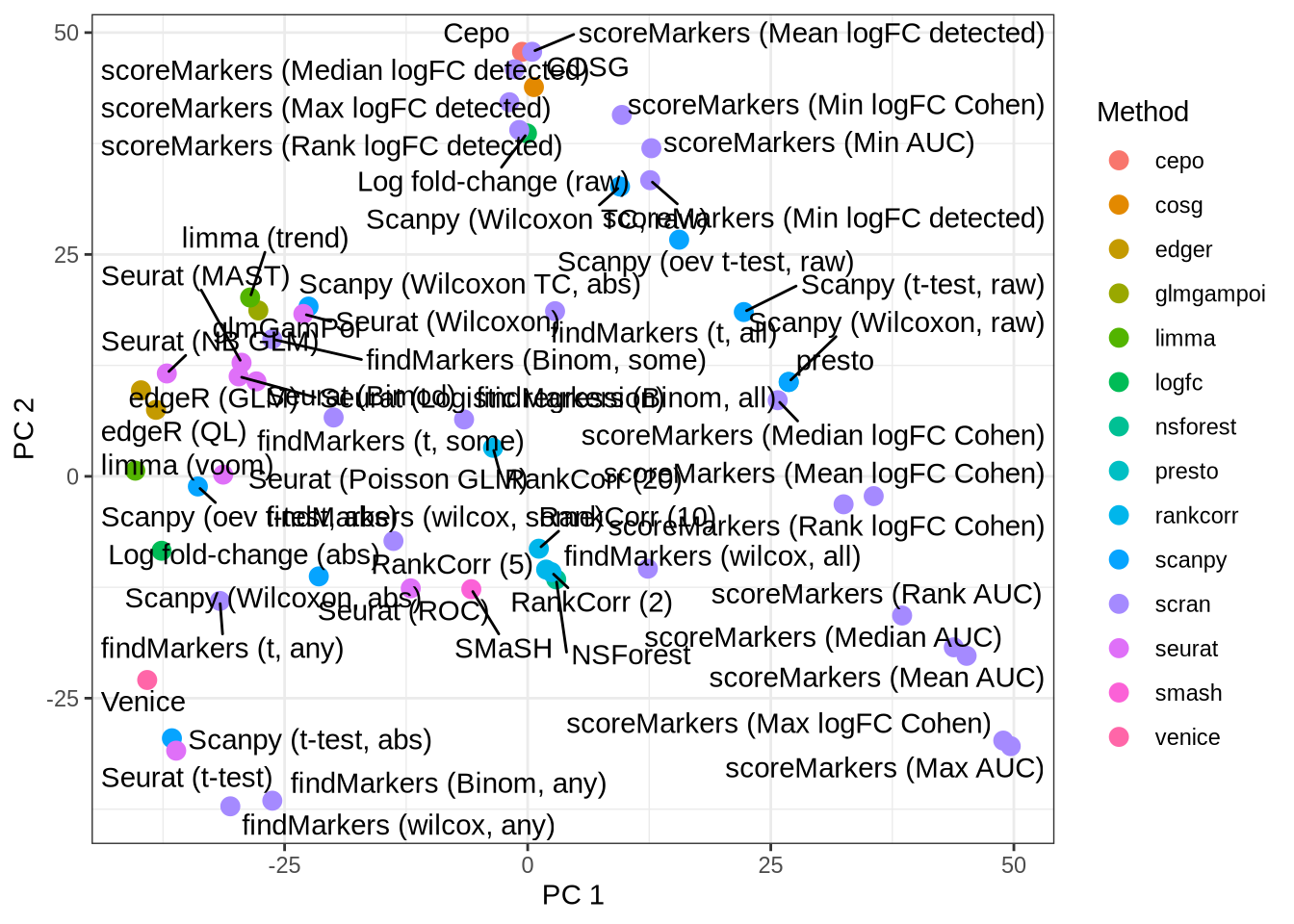

Intersection concordance analysis

all_datasets_results <- load_real_data_results("all")
n_genes <- 20

seurat_results <- all_datasets_results %>% 
  filter(pars == "seurat_wilcox") %>%
  rowwise() %>% 
  mutate(mgs = list(get_top_sel_mgs(mgs, n = n_genes))) %>% 
  ungroup() %>% 
  select(cluster, seurat_mgs = mgs)

scanpy_results <- all_datasets_results %>% 
  filter(pars == "scanpy_t_rankby_raw") %>% 
  rowwise() %>% 
  mutate(mgs = list(get_top_sel_mgs(mgs, n = n_genes))) %>% 
  ungroup() %>% 
  select(cluster, scanpy_mgs = mgs, data_id)

scanpy_seurat_intersection_plot <- seurat_results %>% 
  left_join(scanpy_results, by = "cluster") %>% 
  rowwise() %>% 
  mutate(
    prop_intersect = length(intersect(seurat_mgs$gene, scanpy_mgs$gene)) / n_genes
  ) %>% 
  ungroup() %>% 
  mutate(plot_data_id = dataset_lookup[data_id]) %>% 
  mutate(plot_data_id = fct_reorder(factor(plot_data_id), prop_intersect)) %>% 
  ggplot(aes(x = plot_data_id, y = prop_intersect)) + 
  geom_boxplot(outlier.shape = NA) + 
  geom_jitter(size = 2, width = 0.1, colour = "forestgreen") + 
  coord_flip(ylim = c(0, 1)) + 
  labs(
    x = "Dataset", 
    y = "Proportion of shared genes"
  ) + 
  theme_bw()
scanpy_seurat_intersection_plot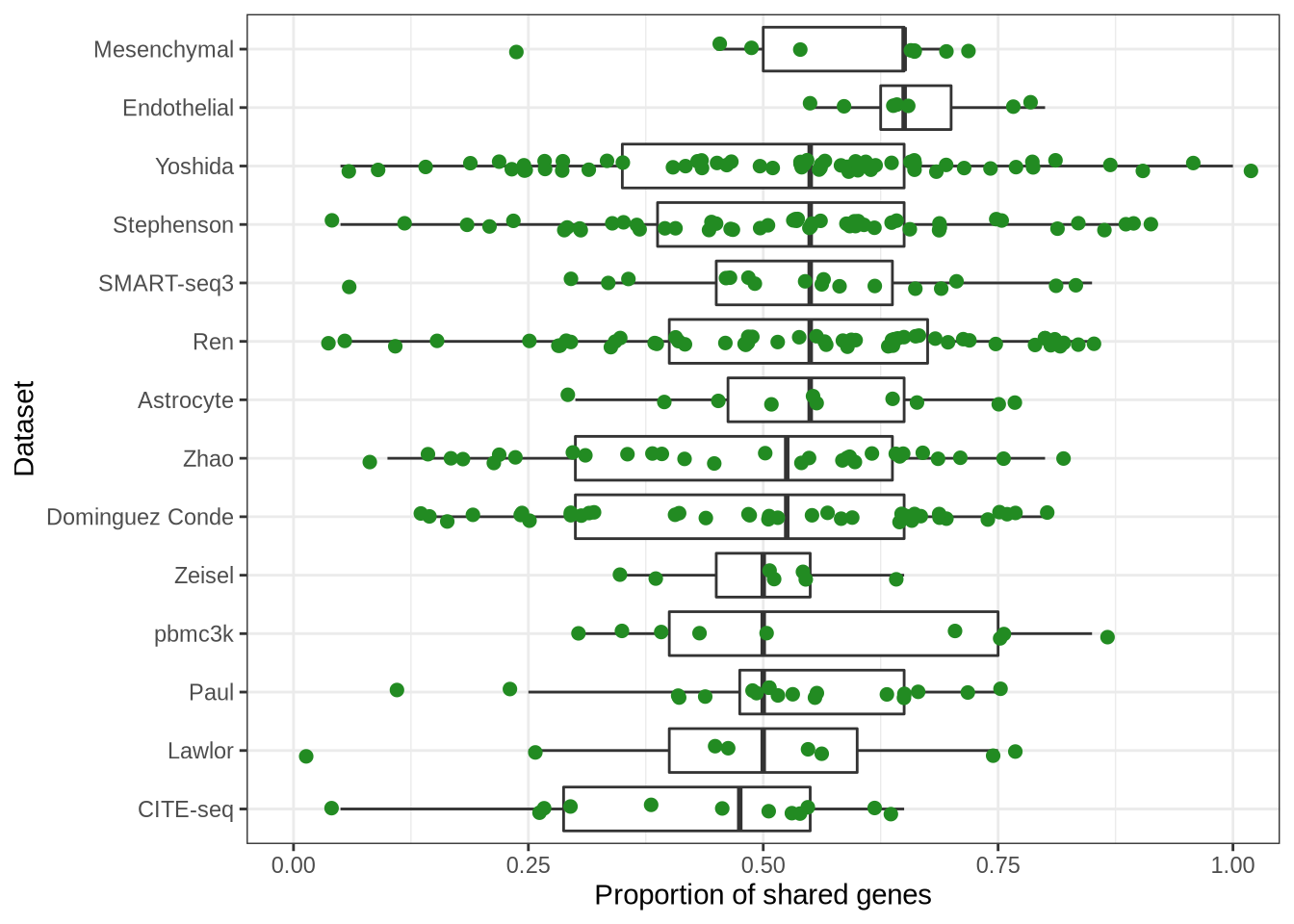

saveRDS(
  scanpy_seurat_intersection_plot,
  here::here("figures", "raw", "scanpy-seurat-intersection.rds")
)

Visual rank concordance analysis

Unless otherwise stated these plots are generated for the B cell cluster in the pbmc3k dataset.

scanpy_t_raw <- readRDS(
  here::here("results", "real_data", "pbmc3k-scanpy_t_rankby_raw.rds")
)

scanpy_t_abs <- readRDS(
  here::here("results", "real_data", "pbmc3k-scanpy_t_rankby_abs.rds")
)

seurat_t <- readRDS(
  here::here("results", "real_data", "pbmc3k-seurat_t.rds")
)

scanpy_wilcox <- readRDS(
  here::here("results", "real_data", "pbmc3k-scanpy_wilcoxon_rankby_raw.rds")
)

scanpy_wilcox_tc <- readRDS(
  here::here("results", "real_data", 
             "pbmc3k-scanpy_wilcoxontiecorrect_rankby_raw.rds")
)

scanpy_wilcox_tc_rankby_abs <- readRDS(
  here::here("results", "real_data", 
             "pbmc3k-scanpy_wilcoxontiecorrect_rankby_abs.rds")
)

seurat_wilcox <- readRDS(
  here::here("results", "real_data", "pbmc3k-seurat_wilcox.rds")
)

scran_t_any <- readRDS(
  here::here("results", "real_data", "pbmc3k-scran_findMarkers_t_any.rds")
)

Seurat default vs Scanpy default

scanpy_default_seurat_default_plot <- rank_rank_plot(
  get_top_marker_genes(scanpy_t_raw, cluster = "CD8 T", n = 20),
  get_top_marker_genes(seurat_wilcox, cluster = "CD8 T", n = 20),
  label1 = "Scanpy default", 
  label2 = "Seurat default"
) +
  ggtitle("Scanpy vs Seurat (CD8 T)") +
  theme(axis.ticks.y = element_blank())

scanpy_default_seurat_default_plot

saveRDS(scanpy_default_seurat_default_plot, 
        here::here("figures", "raw", "rank-rank-scanpy-default-seurat-default.rds"))

Scanpy Wilcox vs Seurat Wilcox

Disagreement caused (mainly) by tie-correction differences and also by regulation ranking differences. (Statistic vs p-value ranking has no effect.)

rank_rank_plot(
  get_top_marker_genes(scanpy_wilcox, cluster = "B", n = 40),
  get_top_marker_genes(seurat_wilcox, cluster = "B", n = 40),
  label1 = "Scanpy Wilcoxon", 
  label2 = "Seurat Wilcoxon"
) + 
  ggtitle("Scanpy Wilcoxon vs Seurat Wilcoxon")

Scanpy tie-corrected Wilcoxon vs Seurat Wilcox

Disagreement caused by regulation ranking difference (Smaller than for t-test due to enrichment for up-regulated genes.)

rank_rank_plot(
  get_top_marker_genes(scanpy_wilcox_tc, cluster = "B", n = 40),
  get_top_marker_genes(seurat_wilcox, cluster = "B", n = 40),
  label1 = "Scanpy Wilcoxon (tie-corrected)", 
  label2 = "Seurat Wilcoxon"
) + 
  ggtitle("Scanpy Wilcoxon (tie-corrected) vs Seurat Wilcoxon")

Scanpy tie-corrected Wilcoxon (ranking by absolute value) vs Seurat Wilcox

Complete agreement. (NB: Two p-values are 0 but the log fold change order is identical to the statistic order, see Zeisel, oligodendrocyte example below.)

rank_rank_plot(
  get_top_marker_genes(scanpy_wilcox_tc_rankby_abs, cluster = "B", n = 40),
  get_top_marker_genes(seurat_wilcox, cluster = "B", n = 40),
  label1 = "Scanpy Wilcoxon (tie-corrected, ranking by absolute value)", 
  label2 = "Seurat Wilcoxon"
) + 
  ggtitle("Scanpy Wilcoxon (tie-corrected, ranking by absolute value) vs Seurat Wilcoxon")

Scanpy t vs Seurat t

Disagreement caused mainly by regulation ranking difference, and issues with ranking by the t-statistic when using Welch’s t-test.

rank_rank_plot(
  get_top_marker_genes(scanpy_t_raw, cluster = "B", n = 40),
  get_top_marker_genes(seurat_t, cluster = "B", n = 40),
  label1 = "Scanpy t", 
  label2 = "Seurat t"
) + 
  ggtitle("Scanpy t vs Seurat t")

Scanpy t (ranking by absolute value) vs Seurat t

Disagreement caused by issues with ranking by the t-statistic when using Welch’s t-test.

rr_scanpy_t_abs_seurat_t <- rank_rank_plot(
  get_top_marker_genes(scanpy_t_abs, cluster = "B", n = 20),
  get_top_marker_genes(seurat_t, cluster = "B", n = 20),
  label1 = "Scanpy t\n(ranking by absolute value)", 
  label2 = "Seurat t"
) + 
  theme(axis.ticks.y = element_blank())

rr_scanpy_t_abs_seurat_t

saveRDS(
  rr_scanpy_t_abs_seurat_t, 
  here::here("figures", "raw", "rr-scanpy-t-abs-seurat-t.rds")
)

Scanpy tie-corrected Wilcoxon (ranking by absolute value) vs Seurat Wilcox (Zeisel data, oligodendrocyte cluster)

Disagreement caused solely difference in p-value vs statistic ranking. The oligodendrocyte cluster has a large number of zero p-values.

zeisel_seurat_wilcox <- readRDS(
  here::here("results", "real_data", "zeisel-seurat_wilcox.rds")
)

zeisel_scanpy_wilcox_tc_abs <- readRDS(
  here::here("results", "real_data",
             "zeisel-scanpy_wilcoxontiecorrect_rankby_abs.rds")
)

n <- 40
cluster <- "oligodendrocytes"
rank_rank_plot(
  get_top_marker_genes(zeisel_seurat_wilcox, cluster = cluster, n = n), 
  get_top_marker_genes(zeisel_scanpy_wilcox_tc_abs, cluster = cluster, n = n), 
  label1 = "Seurat Wilcoxon", 
  label2 = "Scanpy Wilcoxon (tie corrected, ranking by absolute value)"
) + 
  ggtitle("Scanpy Wilcoxon (tie-corrected, ranking by absolute value) vs Seurat Wilcoxon")

Load simulated data

n_cells_data <- retrive_simulation_parameters() %>% 
  filter(sim_label == "num_cells") %>% 
  rowwise() %>% 
  mutate(
    mgs_raw = list(readRDS(full_filename)$result), 
    mgs = list(split(mgs_raw, mgs_raw$cluster))
  ) %>% 
  ungroup() %>% 
  unnest_longer(
    col = mgs, 
    values_to = "mgs", 
    indices_to = "cluster"
  ) %>% 
  select(-mgs_raw)

Log fold-change concordance

n <- 20

logfc_mgs <- n_cells_data %>% 
  filter(cluster == "Group2", rep == 1) %>% 
  filter(pars %in% "logfc_raw") %>%
  rowwise() %>% 
  mutate(mgs = list(get_top_sel_mgs(mgs, n))) %>% 
  ungroup() %>% 
  select(logfc_mgs = mgs, batchCells)

rest_mgs <- n_cells_data %>% 
  filter(cluster == "Group2", rep == 1) %>% 
  filter(method %in% c("seurat", "scanpy")) %>%
  # We do not see the effect for ROC because it does not sort by p-value.
  filter(pars != "seurat_roc") %>% 
  # The GLM use a differently calculated log-fc statistic. 
  filter(!(pars %in% c("seurat_negbinom", "seurat_poisson"))) %>% 
  rowwise() %>% 
  mutate(mgs = list(get_top_sel_mgs(mgs, n))) %>% 
  ungroup() %>% 
  dplyr::rename(other_mgs = mgs)

logfc_abs_prop_intersect_plot <- rest_mgs %>% 
  left_join(logfc_mgs, by = "batchCells") %>% 
  rowwise() %>% 
  mutate(
    prop_intersect = length(intersect(logfc_mgs$gene, other_mgs$gene)) / n
  ) %>% 
  mutate(plot_method = method_lookup[method]) %>% 
  ungroup() %>% 
  ggplot(aes(x = factor(batchCells), y = prop_intersect, 
             fill = factor(plot_method))) + 
  geom_boxplot() + 
  coord_cartesian(ylim = c(0.5, 1)) +
  labs(
    x = "Total cells simulated", 
    y = "Intersection with raw log fold-change method",
    fill = "Package"
  ) + 
  scale_fill_manual(values = c("#1e90ff", "#ff0000")) + 
  theme_bw()
logfc_abs_prop_intersect_plot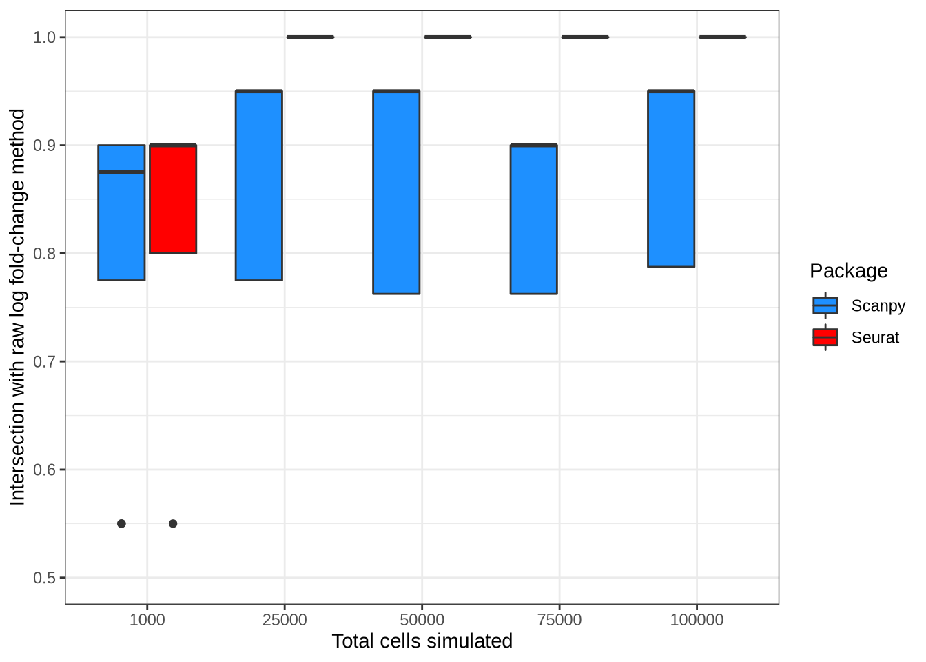

saveRDS(
  logfc_abs_prop_intersect_plot, 
  here::here("figures", "raw", "logfc-abs-prop-intersect.rds")
)

plot_dendrogram_by_dataset <- function(data, data_id) {
  
  n <- 10
  all_concordance_data <- data %>% 
    filter(data_id == !!data_id) %>% 
    rowwise() %>% 
    mutate(mgs = list(get_top_sel_mgs(mgs, n = n)$gene)) %>% 
    ungroup() %>% 
    select(pars, method, cluster, data_id, mgs)
  
  intersection_data <- all_concordance_data %>% 
    expand_grid(pars_2 = unique(all_concordance_data$pars)) %>% 
    left_join(
      dplyr::rename(all_concordance_data, mgs_2 = mgs), 
      by = c("pars_2" = "pars", "cluster")
    ) %>% 
    rowwise() %>% 
    mutate(prop_intersect = length(intersect(mgs, mgs_2)) / n) %>% 
    ungroup() %>% 
    select(pars, pars_2, cluster, prop_intersect)  %>%
    group_by(pars, pars_2) %>% 
    summarise(prop_intersect = mean(prop_intersect), .groups = "drop") %>% 
    pivot_wider(names_from = pars, values_from = prop_intersect)
  
  intersection_mat <- as.matrix(intersection_data[, -1])
  rownames(intersection_mat) <- intersection_data[[1]]
  
  hier_clust <- hclust(dist(intersection_mat))
  hier_clust$labels <- pars_lookup[hier_clust$labels]
  
  hier_clust_data <- dendro_data(hier_clust, type = "rectangle")
  
  dendrogram_plot <- ggplot() +
    geom_segment(data = segment(hier_clust_data), 
                 aes(x = x, y = y, xend = xend, yend = yend)
    ) +
    geom_text(data = label(hier_clust_data), 
              aes(x = x, y = y, label = label, hjust = 0), 
              size = 4
    ) +
    coord_flip(xlim = c(3, 57)) +
    scale_y_reverse(limits = c(4, -1.5)) + 
    theme_dendro()
  
  dendrogram_plot
}

pbmc3k_dendro <- plot_dendrogram_by_dataset(concordance_data, "pbmc3k") + 
  ggtitle("pbmc3k")
endothelial_dendro <- plot_dendrogram_by_dataset(concordance_data, "endothelial") + 
  ggtitle("Endothelial")
ren_dendro <- plot_dendrogram_by_dataset(concordance_data, "ren") + 
  ggtitle("Ren")
astrocyte_dendro <- plot_dendrogram_by_dataset(concordance_data, "astrocyte") + 
  ggtitle("Astrocyte")

dataset_dendro <- pbmc3k_dendro + endothelial_dendro + ren_dendro + 
  astrocyte_dendro + 
  plot_layout(guides = "collect") +
  plot_annotation(tag_levels = "a") &
  theme(plot.tag = element_text(size = 18))

ggsave(
  filename = here::here("figures", "final", "dataset-dendro.pdf"),
  plot = dataset_dendro,
  width = 14,
  height = 18,
  units = "in"
)

n_cells_data <- lapply(
  list.files(here::here("data", "real_data"), full.names = TRUE), 
  function(x) {
   data <- readRDS(x)
   out <- tibble(
     data_id = tools::file_path_sans_ext(basename(x)),
     cell_type = unique(data$label),
     n = as.vector(table(data$label))
   )
   rm(data)
   out
  }
) %>% 
  bind_rows(!!!.)

n <- 10
all_concordance_data <- concordance_data %>% 
  rowwise() %>% 
  mutate(mgs = list(get_top_sel_mgs(mgs, n = n)$gene)) %>% 
  ungroup() %>% 
  select(pars, method, cluster, data_id, mgs)

intersect_n_cells_data <- all_concordance_data %>% 
  expand_grid(pars_2 = unique(all_concordance_data$pars)) %>% 
  left_join(
    dplyr::rename(all_concordance_data, mgs_2 = mgs), 
    by = c("pars_2" = "pars", "cluster")
  ) %>% 
  rowwise() %>% 
  mutate(prop_intersect = length(intersect(mgs, mgs_2)) / n) %>% 
  ungroup() %>% 
  select(pars, pars_2, cluster, prop_intersect, data_id.x)  %>%
  group_by(cluster, data_id.x) %>% 
  summarise(prop_intersect = mean(prop_intersect), .groups = "drop") %>% 
  left_join(n_cells_data, by = c("cluster" = "cell_type", "data_id.x" = "data_id"))

intersect_n_cells_plot <- intersect_n_cells_data %>% 
  filter(!is.na(n)) %>% 
  ggplot(aes(n, prop_intersect)) + 
  geom_point() + 
  labs(
    x = "Number of cells", 
    y = "Intersect proportion"
  ) + 
  theme_bw()

ggsave(
  filename = here::here("figures", "final", "intersect-n-cells.pdf"),
  plot = intersect_n_cells_plot ,
  width = 8,
  height = 8,
  units = "in"
)

Session information

devtools::session_info()

─ Session info  ──────────────────────────────────────────────────────────────
 hash: person frowning: dark skin tone, elevator, right-facing fist: medium-dark skin tone

 setting  value
 version  R version 4.1.2 (2021-11-01)
 os       Red Hat Enterprise Linux 9.2 (Plow)
 system   x86_64, linux-gnu
 ui       X11
 language (EN)
 collate  en_AU.UTF-8
 ctype    en_AU.UTF-8
 tz       Australia/Melbourne
 date     2024-01-01
 pandoc   2.18 @ /apps/easybuild-2022/easybuild/software/MPI/GCC/11.3.0/OpenMPI/4.1.4/RStudio-Server/2022.07.2+576-Java-11-R-4.1.2/bin/pandoc/ (via rmarkdown)

─ Packages ───────────────────────────────────────────────────────────────────
 package              * version  date (UTC) lib source
 assertthat             0.2.1    2019-03-21 [2] CRAN (R 4.1.2)
 beachmat               2.10.0   2021-10-26 [1] Bioconductor
 beeswarm               0.4.0    2021-06-01 [2] CRAN (R 4.1.2)
 Biobase              * 2.54.0   2021-10-26 [1] Bioconductor
 BiocGenerics         * 0.40.0   2021-10-26 [1] Bioconductor
 BiocNeighbors          1.12.0   2021-10-26 [1] Bioconductor
 BiocParallel           1.28.3   2021-12-09 [1] Bioconductor
 BiocSingular           1.10.0   2021-10-26 [1] Bioconductor
 bitops                 1.0-7    2021-04-24 [2] CRAN (R 4.1.2)
 bslib                  0.3.1    2021-10-06 [1] CRAN (R 4.1.0)
 cachem                 1.0.6    2021-08-19 [1] CRAN (R 4.1.0)
 callr                  3.7.0    2021-04-20 [2] CRAN (R 4.1.2)
 cli                    3.6.1    2023-03-23 [1] CRAN (R 4.1.0)
 colorspace             2.1-0    2023-01-23 [1] CRAN (R 4.1.0)
 crayon                 1.5.1    2022-03-26 [1] CRAN (R 4.1.0)
 DBI                    1.1.2    2021-12-20 [1] CRAN (R 4.1.0)
 DelayedArray           0.20.0   2021-10-26 [1] Bioconductor
 DelayedMatrixStats     1.16.0   2021-10-26 [1] Bioconductor
 desc                   1.4.0    2021-09-28 [2] CRAN (R 4.1.2)
 devtools               2.4.2    2021-06-07 [2] CRAN (R 4.1.2)
 dichromat              2.0-0    2013-01-24 [2] CRAN (R 4.1.2)
 digest                 0.6.29   2021-12-01 [1] CRAN (R 4.1.0)
 dplyr                * 1.0.9    2022-04-28 [1] CRAN (R 4.1.0)
 ellipsis               0.3.2    2021-04-29 [2] CRAN (R 4.1.2)
 evaluate               0.14     2019-05-28 [2] CRAN (R 4.1.2)
 fansi                  1.0.4    2023-01-22 [1] CRAN (R 4.1.0)
 farver                 2.1.1    2022-07-06 [1] CRAN (R 4.1.0)
 fastmap                1.1.0    2021-01-25 [2] CRAN (R 4.1.2)
 forcats              * 0.5.1    2021-01-27 [2] CRAN (R 4.1.2)
 fs                     1.5.2    2021-12-08 [1] CRAN (R 4.1.0)
 generics               0.1.3    2022-07-05 [1] CRAN (R 4.1.0)
 GenomeInfoDb         * 1.30.0   2021-10-26 [1] Bioconductor
 GenomeInfoDbData       1.2.7    2021-12-03 [1] Bioconductor
 GenomicRanges        * 1.46.1   2021-11-18 [1] Bioconductor
 ggbeeswarm             0.6.0    2017-08-07 [2] CRAN (R 4.1.2)
 ggdendro             * 0.1.23   2022-02-16 [1] CRAN (R 4.1.0)
 ggplot2              * 3.3.6    2022-05-03 [1] CRAN (R 4.1.0)
 ggrepel              * 0.9.1    2021-01-15 [2] CRAN (R 4.1.2)
 ggupset              * 0.3.0    2020-05-05 [1] CRAN (R 4.1.0)
 git2r                  0.28.0   2021-01-10 [2] CRAN (R 4.1.2)
 glue                   1.6.0    2021-12-17 [1] CRAN (R 4.1.0)
 gridExtra              2.3      2017-09-09 [2] CRAN (R 4.1.2)
 gtable                 0.3.0    2019-03-25 [2] CRAN (R 4.1.2)
 here                   1.0.1    2020-12-13 [1] CRAN (R 4.1.0)
 highr                  0.9      2021-04-16 [2] CRAN (R 4.1.2)
 htmltools              0.5.2    2021-08-25 [1] CRAN (R 4.1.0)
 httpuv                 1.6.5    2022-01-05 [1] CRAN (R 4.1.0)
 IRanges              * 2.28.0   2021-10-26 [1] Bioconductor
 irlba                  2.3.5    2021-12-06 [1] CRAN (R 4.1.0)
 jquerylib              0.1.4    2021-04-26 [2] CRAN (R 4.1.2)
 jsonlite               1.8.0    2022-02-22 [1] CRAN (R 4.1.0)
 knitr                  1.36     2021-09-29 [1] CRAN (R 4.1.0)
 labeling               0.4.2    2020-10-20 [2] CRAN (R 4.1.2)
 later                  1.3.0    2021-08-18 [1] CRAN (R 4.1.0)
 lattice                0.20-45  2021-09-22 [2] CRAN (R 4.1.2)
 lifecycle              1.0.1    2021-09-24 [1] CRAN (R 4.1.0)
 logisticPCA          * 0.2      2016-03-14 [1] CRAN (R 4.1.0)
 magrittr               2.0.3    2022-03-30 [1] CRAN (R 4.1.0)
 mapproj                1.2.7    2020-02-03 [1] CRAN (R 4.1.0)
 maps                   3.4.0    2021-09-25 [2] CRAN (R 4.1.2)
 MASS                   7.3-54   2021-05-03 [2] CRAN (R 4.1.2)
 Matrix                 1.3-4    2021-06-01 [2] CRAN (R 4.1.2)
 MatrixGenerics       * 1.6.0    2021-10-26 [1] Bioconductor
 matrixStats          * 0.62.0   2022-04-19 [1] CRAN (R 4.1.0)
 memoise                2.0.1    2021-11-26 [1] CRAN (R 4.1.0)
 munsell                0.5.0    2018-06-12 [2] CRAN (R 4.1.2)
 pals                 * 1.7      2021-04-17 [1] CRAN (R 4.1.0)
 patchwork            * 1.1.1    2020-12-17 [2] CRAN (R 4.1.2)
 pillar                 1.7.0    2022-02-01 [1] CRAN (R 4.1.0)
 pkgbuild               1.2.0    2020-12-15 [2] CRAN (R 4.1.2)
 pkgconfig              2.0.3    2019-09-22 [2] CRAN (R 4.1.2)
 pkgload                1.2.3    2021-10-13 [2] CRAN (R 4.1.2)
 prettyunits            1.1.1    2020-01-24 [2] CRAN (R 4.1.2)
 processx               3.5.2    2021-04-30 [2] CRAN (R 4.1.2)
 promises               1.2.0.1  2021-02-11 [2] CRAN (R 4.1.2)
 ps                     1.7.1    2022-06-18 [1] CRAN (R 4.1.0)
 purrr                * 0.3.4    2020-04-17 [2] CRAN (R 4.1.2)
 R6                     2.5.1    2021-08-19 [1] CRAN (R 4.1.0)
 Rcpp                   1.0.8.3  2022-03-17 [1] CRAN (R 4.1.0)
 RCurl                  1.98-1.5 2021-09-17 [1] CRAN (R 4.1.0)
 remotes                2.4.2    2021-11-30 [1] CRAN (R 4.1.0)
 rlang                  1.0.3    2022-06-27 [1] CRAN (R 4.1.0)
 rmarkdown              2.14     2022-04-25 [1] CRAN (R 4.1.0)
 rprojroot              2.0.3    2022-04-02 [1] CRAN (R 4.1.0)
 rstudioapi             0.14     2022-08-22 [1] CRAN (R 4.1.0)
 rsvd                   1.0.5    2021-04-16 [1] CRAN (R 4.1.0)
 S4Vectors            * 0.32.3   2021-11-21 [1] Bioconductor
 sass                   0.4.1    2022-03-23 [1] CRAN (R 4.1.0)
 ScaledMatrix           1.2.0    2021-10-26 [1] Bioconductor
 scales                 1.2.1    2022-08-20 [1] CRAN (R 4.1.0)
 scater               * 1.22.0   2021-10-26 [1] Bioconductor
 scuttle              * 1.4.0    2021-10-26 [1] Bioconductor
 sessioninfo            1.2.0    2021-10-31 [2] CRAN (R 4.1.2)
 SingleCellExperiment * 1.16.0   2021-10-26 [1] Bioconductor
 sparseMatrixStats      1.6.0    2021-10-26 [1] Bioconductor
 stringi                1.7.6    2021-11-29 [1] CRAN (R 4.1.0)
 stringr                1.4.0    2019-02-10 [2] CRAN (R 4.1.2)
 SummarizedExperiment * 1.24.0   2021-10-26 [1] Bioconductor
 testthat               3.1.0    2021-10-04 [2] CRAN (R 4.1.2)
 tibble               * 3.1.7    2022-05-03 [1] CRAN (R 4.1.0)
 tidyr                * 1.2.0    2022-02-01 [1] CRAN (R 4.1.0)
 tidyselect             1.1.2    2022-02-21 [1] CRAN (R 4.1.0)
 topconfects          * 1.10.0   2021-10-26 [1] Bioconductor
 usethis                2.1.3    2021-10-27 [2] CRAN (R 4.1.2)
 utf8                   1.2.3    2023-01-31 [1] CRAN (R 4.1.0)
 vctrs                  0.4.1    2022-04-13 [1] CRAN (R 4.1.0)
 vipor                  0.4.5    2017-03-22 [2] CRAN (R 4.1.2)
 viridis                0.6.2    2021-10-13 [1] CRAN (R 4.1.0)
 viridisLite            0.4.2    2023-05-02 [1] CRAN (R 4.1.0)
 whisker                0.4      2019-08-28 [2] CRAN (R 4.1.2)
 withr                  2.5.0    2022-03-03 [1] CRAN (R 4.1.0)
 workflowr              1.7.0    2021-12-21 [1] CRAN (R 4.1.0)
 xfun                   0.31     2022-05-10 [1] CRAN (R 4.1.0)
 XVector                0.34.0   2021-10-26 [1] Bioconductor
 yaml                   2.3.5    2022-02-21 [1] CRAN (R 4.1.0)
 zlibbioc               1.40.0   2021-10-26 [1] Bioconductor

 [1] /home/jpullin/R/x86_64-pc-linux-gnu-library/4.1
 [2] /apps/easybuild-2022/easybuild/software/MPI/GCC/11.3.0/OpenMPI/4.1.4/R/4.1.2/lib64/R/library

──────────────────────────────────────────────────────────────────────────────