Simualted data analysis
Last updated: 2024-01-01
Checks: 7 0
Knit directory:
mage_2020_marker-gene-benchmarking/
This reproducible R Markdown analysis was created with workflowr (version 1.7.0). The Checks tab describes the reproducibility checks that were applied when the results were created. The Past versions tab lists the development history.
Great! Since the R Markdown file has been committed to the Git repository, you know the exact version of the code that produced these results.
Great job! The global environment was empty. Objects defined in the global environment can affect the analysis in your R Markdown file in unknown ways. For reproduciblity it’s best to always run the code in an empty environment.
The command set.seed(20190102) was run prior to running
the code in the R Markdown file. Setting a seed ensures that any results
that rely on randomness, e.g. subsampling or permutations, are
reproducible.
Great job! Recording the operating system, R version, and package versions is critical for reproducibility.
Nice! There were no cached chunks for this analysis, so you can be confident that you successfully produced the results during this run.
Great job! Using relative paths to the files within your workflowr project makes it easier to run your code on other machines.
Great! You are using Git for version control. Tracking code development and connecting the code version to the results is critical for reproducibility.
The results in this page were generated with repository version 2632193. See the Past versions tab to see a history of the changes made to the R Markdown and HTML files.
Note that you need to be careful to ensure that all relevant files for
the analysis have been committed to Git prior to generating the results
(you can use wflow_publish or
wflow_git_commit). workflowr only checks the R Markdown
file, but you know if there are other scripts or data files that it
depends on. Below is the status of the Git repository when the results
were generated:
Ignored files:
    Ignored:    .Renviron
    Ignored:    .Rhistory
    Ignored:    .Rproj.user/
    Ignored:    .snakemake/
    Ignored:    NSForest/.Rhistory
    Ignored:    NSForest/NS-Forest_v3_Extended_Binary_Markers_Supplmental.csv
    Ignored:    NSForest/NS-Forest_v3_Full_Results.csv
    Ignored:    NSForest/NSForest3_medianValues.csv
    Ignored:    NSForest/NSForest_v3_Final_Result.csv
    Ignored:    NSForest/__pycache__/
    Ignored:    NSForest/data/
    Ignored:    RankCorr/picturedRocks/__pycache__/
    Ignored:    benchmarks/
    Ignored:    config/
    Ignored:    data/cellmarker/
    Ignored:    data/downloaded_data/
    Ignored:    data/expert_annotations/
    Ignored:    data/expert_mgs/
    Ignored:    data/raw_data/
    Ignored:    data/real_data/
    Ignored:    data/sim_data/
    Ignored:    data/sim_mgs/
    Ignored:    data/special_real_data/
    Ignored:    figures/
    Ignored:    logs/
    Ignored:    results/
    Ignored:    weights/

Unstaged changes:
    Deleted:    analysis/expert-mgs-direction.Rmd
    Modified:   smash-fork
Note that any generated files, e.g. HTML, png, CSS, etc., are not included in this status report because it is ok for generated content to have uncommitted changes.
These are the previous versions of the repository in which changes were
made to the R Markdown
(analysis/simulated-data-analysis.Rmd) and HTML
(public/simulated-data-analysis.html) files. If you’ve
configured a remote Git repository (see ?wflow_git_remote),
click on the hyperlinks in the table below to view the files as they
were in that past version.
| File | Version | Author | Date | Message |
|---|---|---|---|---|
| html | fcecf65 | Jeffrey Pullin | 2022-09-09 | Build site. |
| html | af96b34 | Jeffrey Pullin | 2022-08-30 | Build site. |
| html | 0e47874 | Jeffrey Pullin | 2022-05-04 | Build site. |
| html | 8b989e1 | Jeffrey Pullin | 2022-05-02 | Build site. |
| Rmd | d9e0eb8 | Jeffrey Pullin | 2022-03-28 | Economise simulated data analyses |
library(SingleCellExperiment)Loading required package: SummarizedExperimentLoading required package: MatrixGenericsLoading required package: matrixStats
Attaching package: 'MatrixGenerics'The following objects are masked from 'package:matrixStats':
colAlls, colAnyNAs, colAnys, colAvgsPerRowSet, colCollapse,
colCounts, colCummaxs, colCummins, colCumprods, colCumsums,
colDiffs, colIQRDiffs, colIQRs, colLogSumExps, colMadDiffs,
colMads, colMaxs, colMeans2, colMedians, colMins, colOrderStats,
colProds, colQuantiles, colRanges, colRanks, colSdDiffs, colSds,
colSums2, colTabulates, colVarDiffs, colVars, colWeightedMads,
colWeightedMeans, colWeightedMedians, colWeightedSds,
colWeightedVars, rowAlls, rowAnyNAs, rowAnys, rowAvgsPerColSet,
rowCollapse, rowCounts, rowCummaxs, rowCummins, rowCumprods,
rowCumsums, rowDiffs, rowIQRDiffs, rowIQRs, rowLogSumExps,
rowMadDiffs, rowMads, rowMaxs, rowMeans2, rowMedians, rowMins,
rowOrderStats, rowProds, rowQuantiles, rowRanges, rowRanks,
rowSdDiffs, rowSds, rowSums2, rowTabulates, rowVarDiffs, rowVars,
rowWeightedMads, rowWeightedMeans, rowWeightedMedians,
rowWeightedSds, rowWeightedVarsLoading required package: GenomicRangesLoading required package: stats4Loading required package: BiocGenerics
Attaching package: 'BiocGenerics'The following objects are masked from 'package:stats':
IQR, mad, sd, var, xtabsThe following objects are masked from 'package:base':
anyDuplicated, append, as.data.frame, basename, cbind, colnames,
dirname, do.call, duplicated, eval, evalq, Filter, Find, get, grep,
grepl, intersect, is.unsorted, lapply, Map, mapply, match, mget,
order, paste, pmax, pmax.int, pmin, pmin.int, Position, rank,
rbind, Reduce, rownames, sapply, setdiff, sort, table, tapply,
union, unique, unsplit, which.max, which.minLoading required package: S4Vectors
Attaching package: 'S4Vectors'The following objects are masked from 'package:base':
expand.grid, I, unnameLoading required package: IRangesLoading required package: GenomeInfoDbLoading required package: BiobaseWelcome to Bioconductor
Vignettes contain introductory material; view with
'browseVignettes()'. To cite Bioconductor, see
'citation("Biobase")', and for packages 'citation("pkgname")'.
Attaching package: 'Biobase'The following object is masked from 'package:MatrixGenerics':
rowMediansThe following objects are masked from 'package:matrixStats':
anyMissing, rowMedianslibrary(scater)Loading required package: scuttleLoading required package: ggplot2library(ggplot2)
library(sparseMatrixStats)
library(dplyr)
Attaching package: 'dplyr'The following object is masked from 'package:Biobase':
combineThe following objects are masked from 'package:GenomicRanges':
intersect, setdiff, unionThe following object is masked from 'package:GenomeInfoDb':
intersectThe following objects are masked from 'package:IRanges':
collapse, desc, intersect, setdiff, slice, unionThe following objects are masked from 'package:S4Vectors':
first, intersect, rename, setdiff, setequal, unionThe following objects are masked from 'package:BiocGenerics':
combine, intersect, setdiff, unionThe following object is masked from 'package:matrixStats':
countThe following objects are masked from 'package:stats':
filter, lagThe following objects are masked from 'package:base':
intersect, setdiff, setequal, unionlibrary(scran)
library(purrr)
Attaching package: 'purrr'The following object is masked from 'package:GenomicRanges':
reduceThe following object is masked from 'package:IRanges':
reducesource(here::here("code", "data-analysis-utils.R"))sim_pbmc3k <- readRDS(
here::here("data", "sim_data", "standard_sim_1-pbmc3k.rds")
)plotTSNE(sim_pbmc3k, colour_by = "label") 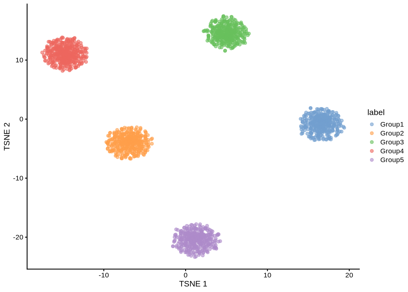
plotUMAP(sim_pbmc3k, colour_by = "label") 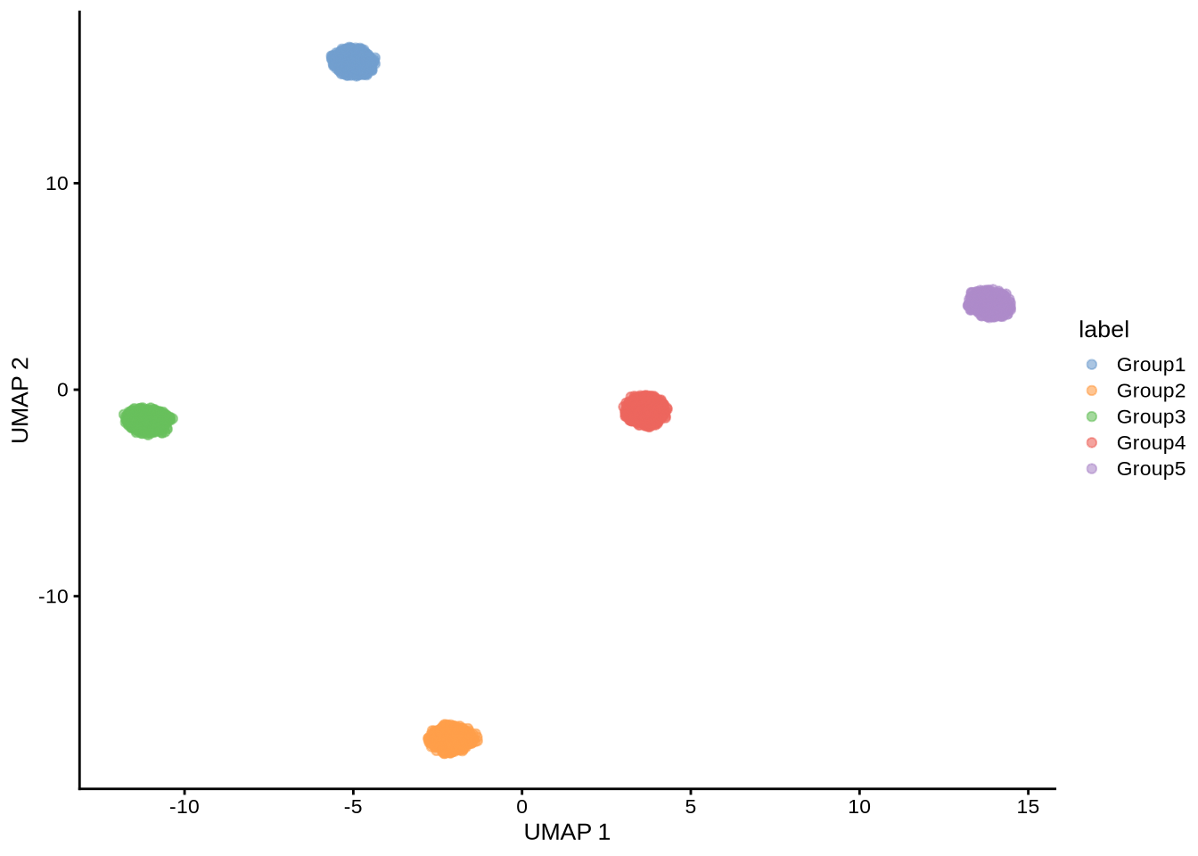
plot_cluster_counts(sim_pbmc3k)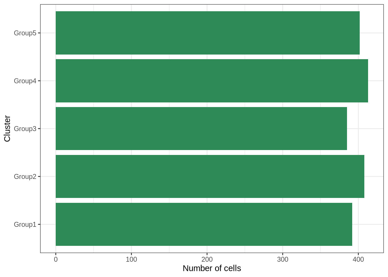
plot_cluster_mean_boxplot(sim_pbmc3k)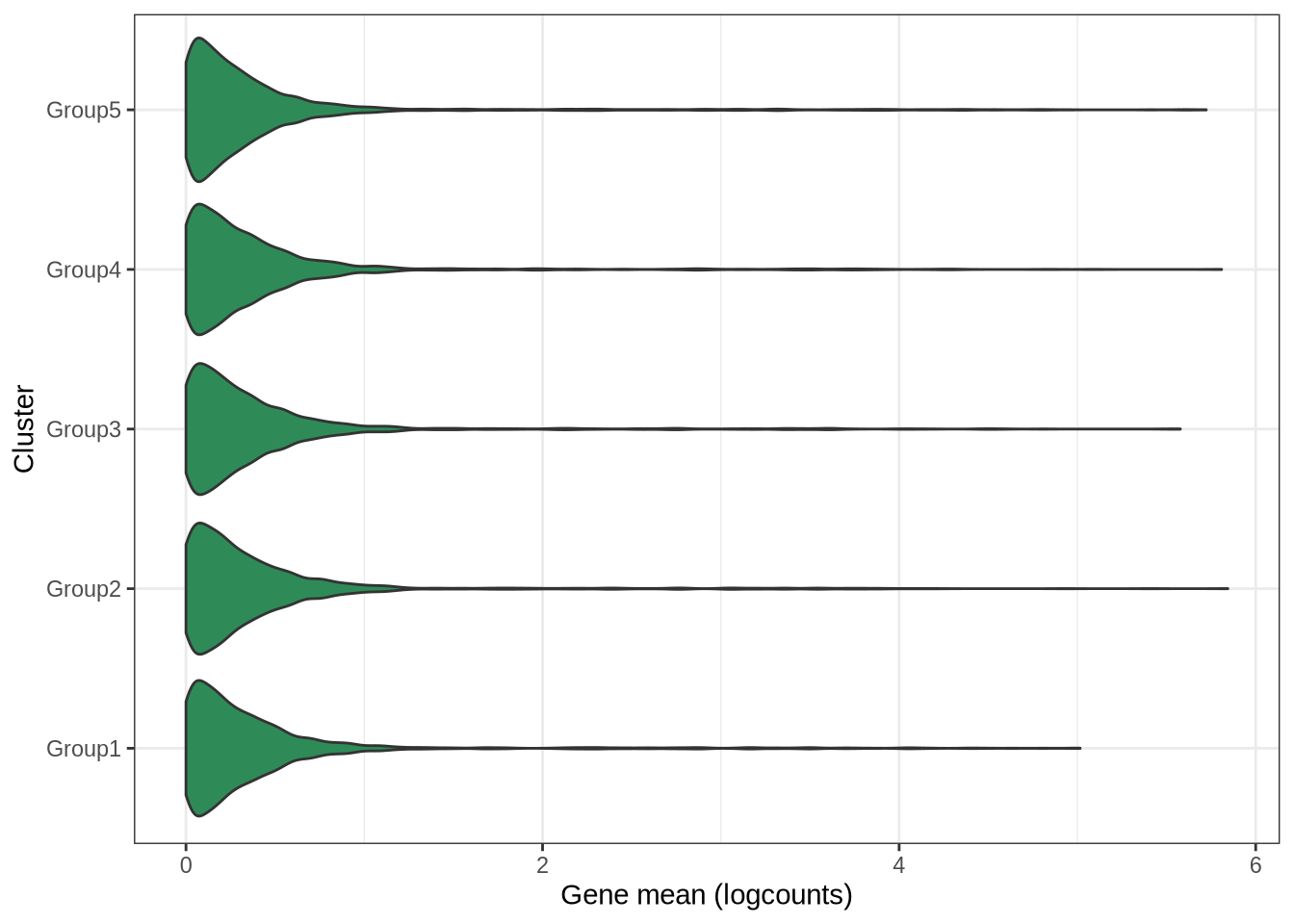
plot_median_diffs(sim_pbmc3k)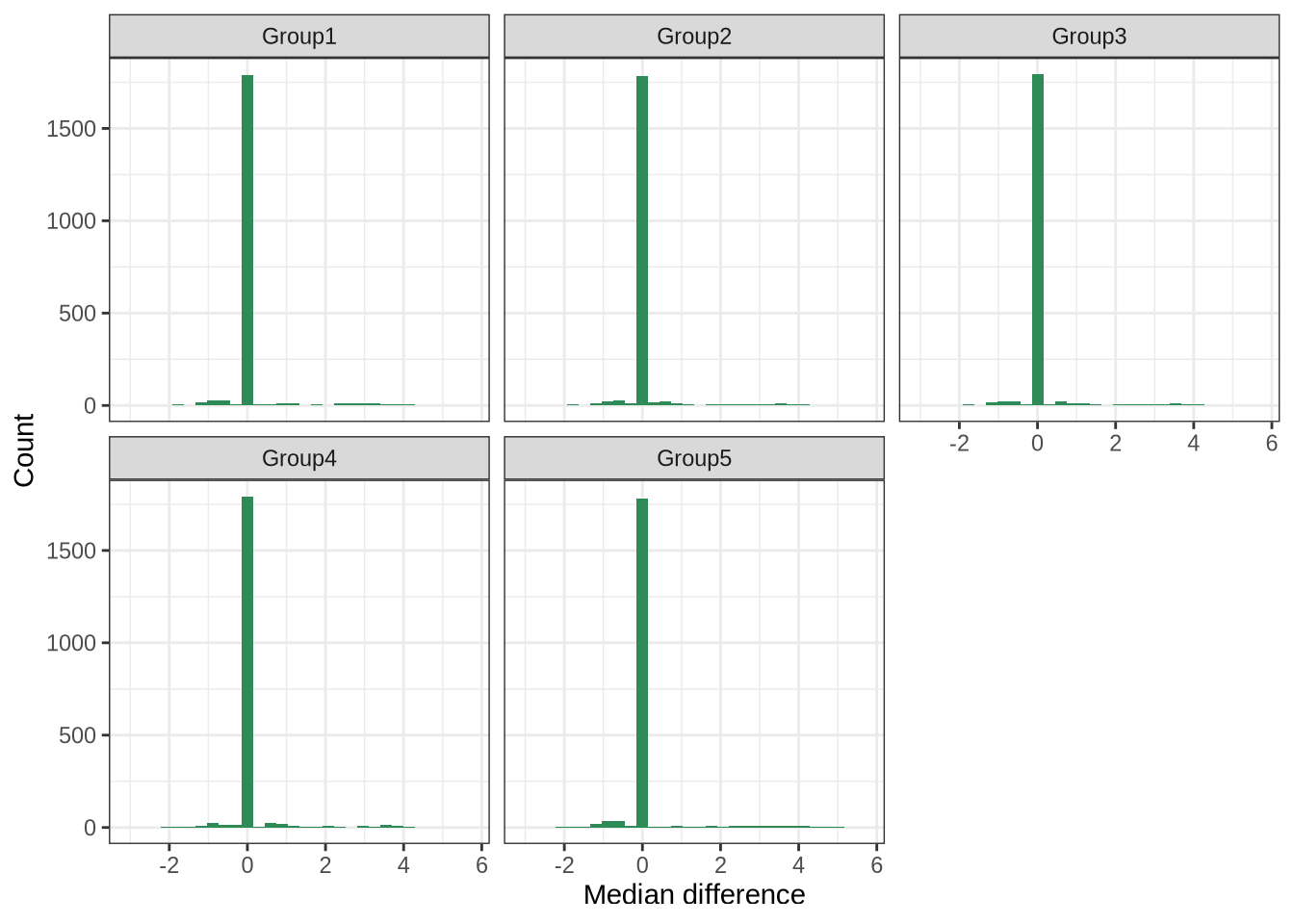
library(ggplot2)ggplot(data.frame(x = 1:40), aes(x)) +
geom_function(fun = ~ dlnorm(.x, 1, 0.2), colour = "red") +
geom_function(fun = ~ dlnorm(.x, 2, 0.2), colour = "blue") +
geom_function(fun = ~ dlnorm(.x, 3, 0.2), colour = "green") +
labs(
title = "Log-normal densities for different parameter values",
x = "x",
y = "Density"
) +
theme_bw()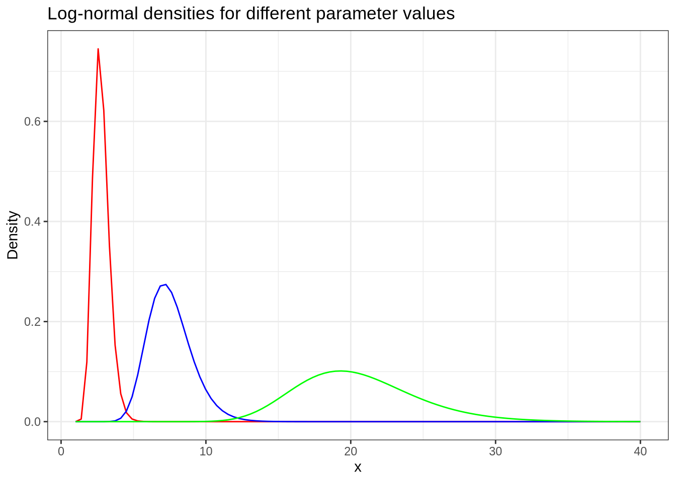
library(splatter)
library(ggplot2)set.seed(42)
# Number of samples to make the histograms from.
N <- 10000default_params <- newSplatParams()
default_params@mean.shape[1] 0.6default_params@mean.rate[1] 0.3default_params <- newSplatParams()
shape <- default_params@mean.shape
rate <- default_params@mean.rate
data.frame(x = rgamma(N, shape = shape, rate = rate)) %>%
ggplot(aes(x)) +
geom_histogram(bins = 50) +
labs(x = "Value", y = "Count") +
theme_bw()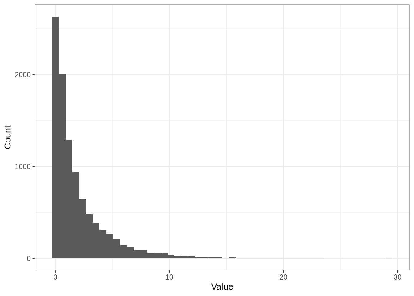
shape[1] 0.6rate[1] 0.3shape / rate[1] 2pbmc <- readRDS(here::here("data", "pbmc3k.rds"))
est_params <- splatEstimate(as.matrix(logcounts(pbmc)))
shape <- est_params@mean.shape
rate <- est_params@mean.rate
data.frame(x = rgamma(N, shape = shape, rate = rate)) %>%
ggplot(aes(x)) +
geom_histogram(bins = 50) +
labs(x = "Value", y = "Count") +
theme_bw()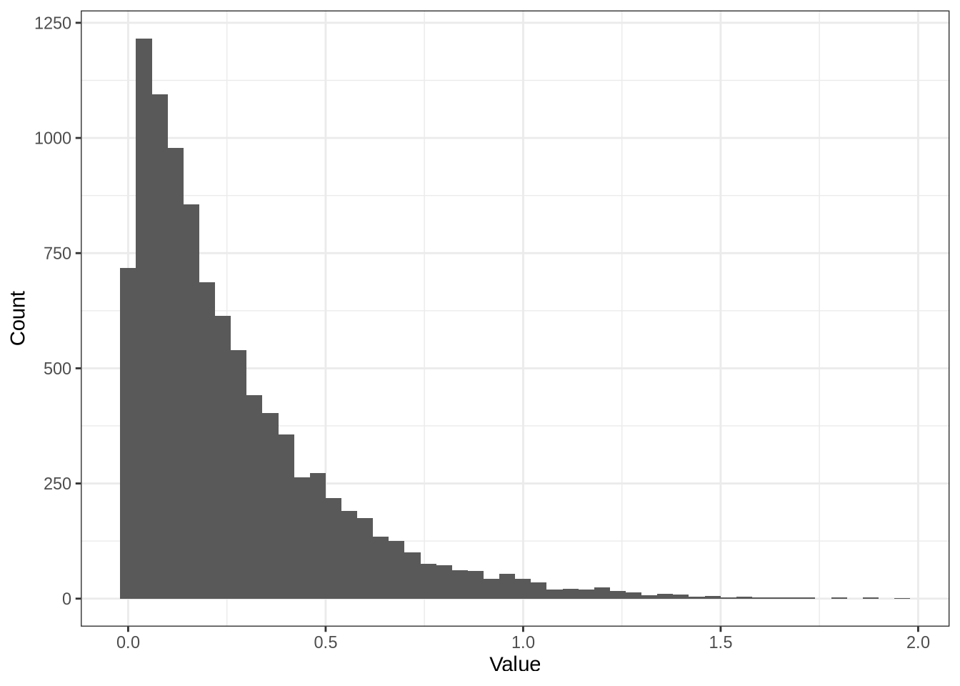
shape[1] 1.028642rate[1] 3.887754shape / rate[1] 0.2645852data.frame(x = seq(1, 10, by = 0.1)) %>%
ggplot(aes(x)) +
geom_function(fun = ~ dgamma(.x, 1, 1)) +
geom_function(fun = ~ dgamma(.x, 1, 2)) +
geom_function(fun = ~ dgamma(.x, 1, 3)) +
geom_function(fun = ~ dgamma(.x, 1, 4))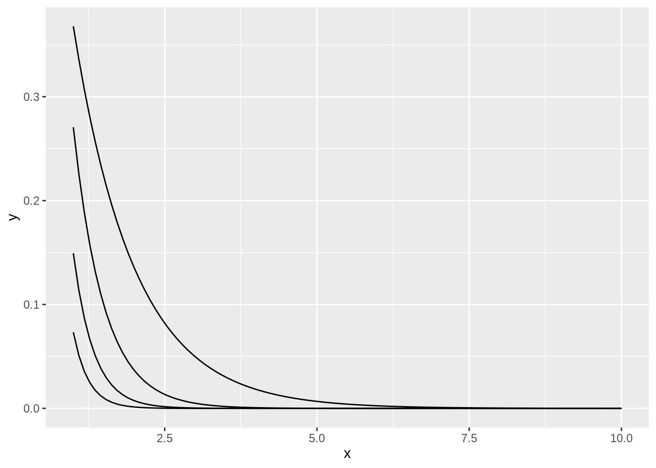
library(splatter)
library(scater)
plot_pca <- function(sce) {
stopifnot(is(sce, "SingleCellExperiment"))
# Calculate logcounts.
sce <- logNormCounts(sce)
sce <- runPCA(sce)
# Cluster the data.
g <- buildSNNGraph(sce, k = , use.dimred = "PCA")
clust <- igraph::cluster_walktrap(g)$membership
colLabels(sce) <- factor(clust)
p <- plotPCA(sce, colour_by = "label")
p
}Aim
Investigate the impact of different parameters, especially those not esimated from real data, on Splatter’s simulations.
Notes
All parameters choices give the same number of unique marker genes.
Baseline
params_sce <- mockSCE()
params <- splatEstimate(params_sce)
NOTE: Library sizes have been found to be normally distributed instead of log-normal. You may want to check this is correct.params@group.prob <- rep(1 / 3, 3)
params@nGroups <- 3sce <- splatSimulateGroups(params)Getting parameters...Creating simulation object...Simulating library sizes...Simulating gene means...Simulating group DE...Simulating cell means...Simulating BCV...Warning in splatSimBCVMeans(sim, params): 'bcv.df' is infinite. This parameter
will be ignored.Simulating counts...Simulating dropout (if needed)...Sparsifying assays...Automatically converting to sparse matrices, threshold = 0.95Skipping 'BatchCellMeans': estimated sparse size 1.5 * dense matrixSkipping 'BaseCellMeans': estimated sparse size 1.5 * dense matrixSkipping 'BCV': estimated sparse size 1.5 * dense matrixSkipping 'CellMeans': estimated sparse size 1.5 * dense matrixSkipping 'TrueCounts': estimated sparse size 2.71 * dense matrixSkipping 'counts': estimated sparse size 2.71 * dense matrixDone!plot_pca(sce)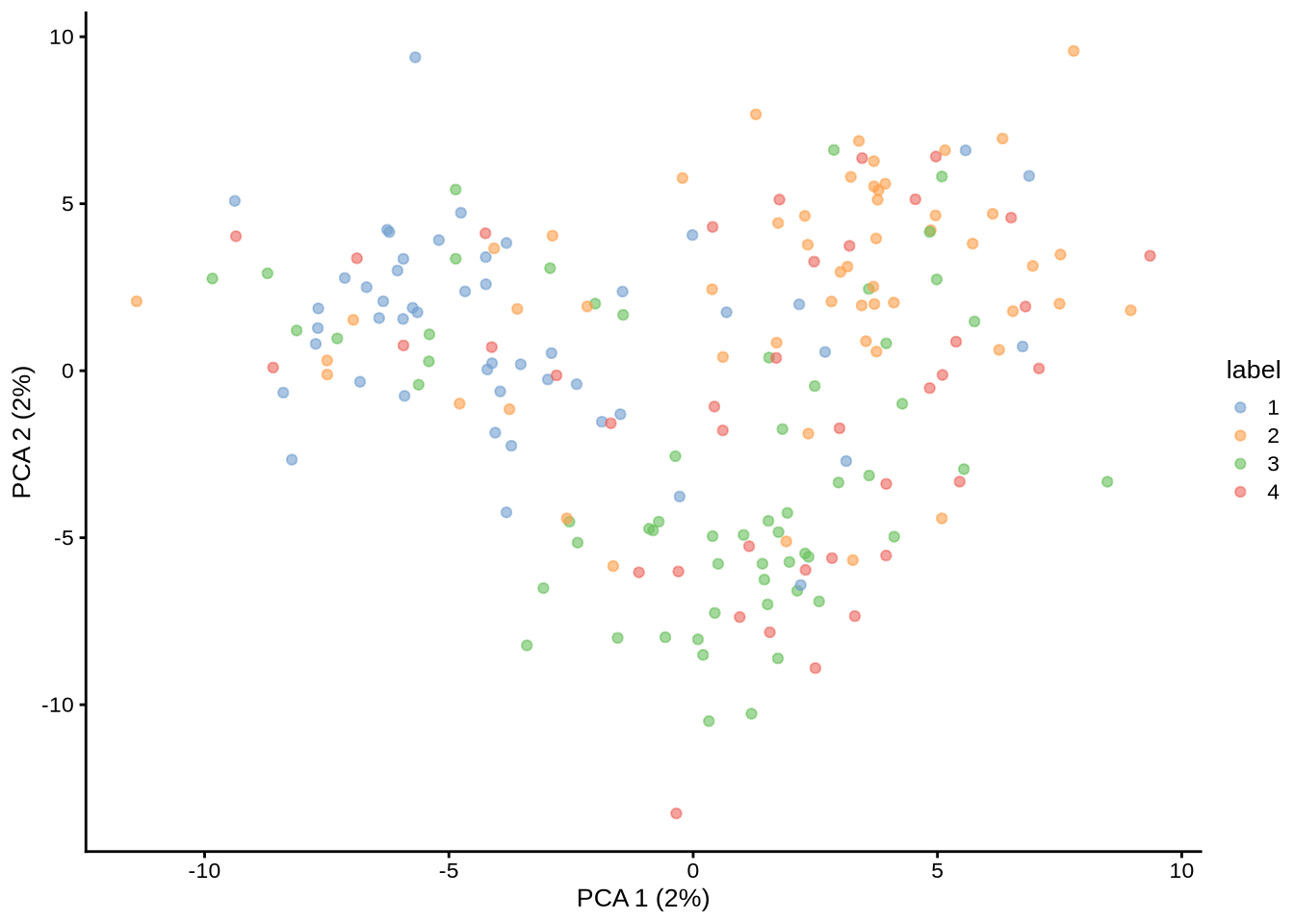
Differential expression location
By default 0.1
params@de.facLoc <- 0.2
sce <- splatSimulateGroups(params)
Getting parameters...Creating simulation object...Simulating library sizes...Simulating gene means...Simulating group DE...Simulating cell means...Simulating BCV...Warning in splatSimBCVMeans(sim, params): 'bcv.df' is infinite. This parameter
will be ignored.Simulating counts...Simulating dropout (if needed)...Sparsifying assays...Automatically converting to sparse matrices, threshold = 0.95Skipping 'BatchCellMeans': estimated sparse size 1.5 * dense matrixSkipping 'BaseCellMeans': estimated sparse size 1.5 * dense matrixSkipping 'BCV': estimated sparse size 1.5 * dense matrixSkipping 'CellMeans': estimated sparse size 1.5 * dense matrixSkipping 'TrueCounts': estimated sparse size 2.71 * dense matrixSkipping 'counts': estimated sparse size 2.71 * dense matrixDone!plot_pca(sce) + ggtitle("de.facLoc = 0.2, 3 groups")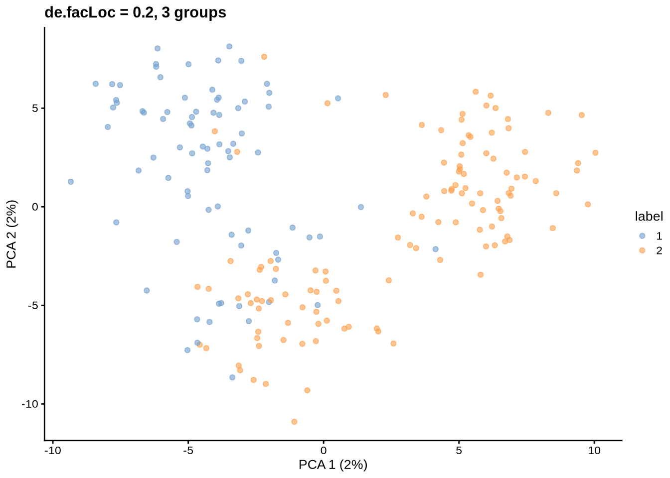
params@de.facLoc <- 0.5
sce <- splatSimulateGroups(params)
Getting parameters...Creating simulation object...Simulating library sizes...Simulating gene means...Simulating group DE...Simulating cell means...Simulating BCV...Warning in splatSimBCVMeans(sim, params): 'bcv.df' is infinite. This parameter
will be ignored.Simulating counts...Simulating dropout (if needed)...Sparsifying assays...Automatically converting to sparse matrices, threshold = 0.95Skipping 'BatchCellMeans': estimated sparse size 1.5 * dense matrixSkipping 'BaseCellMeans': estimated sparse size 1.5 * dense matrixSkipping 'BCV': estimated sparse size 1.5 * dense matrixSkipping 'CellMeans': estimated sparse size 1.5 * dense matrixSkipping 'TrueCounts': estimated sparse size 2.7 * dense matrixSkipping 'counts': estimated sparse size 2.7 * dense matrixDone!plot_pca(sce) + ggtitle("de.facLoc = 0.5, 3 groups")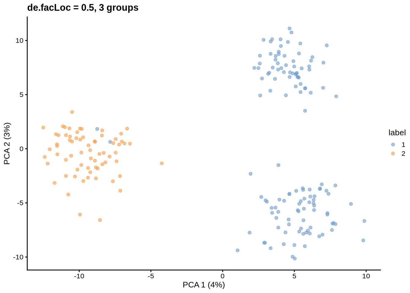
params@de.facLoc <- 1
sce <- splatSimulateGroups(params)
Getting parameters...Creating simulation object...Simulating library sizes...Simulating gene means...Simulating group DE...Simulating cell means...Simulating BCV...Warning in splatSimBCVMeans(sim, params): 'bcv.df' is infinite. This parameter
will be ignored.Simulating counts...Simulating dropout (if needed)...Sparsifying assays...Automatically converting to sparse matrices, threshold = 0.95Skipping 'BatchCellMeans': estimated sparse size 1.5 * dense matrixSkipping 'BaseCellMeans': estimated sparse size 1.5 * dense matrixSkipping 'BCV': estimated sparse size 1.5 * dense matrixSkipping 'CellMeans': estimated sparse size 1.5 * dense matrixSkipping 'TrueCounts': estimated sparse size 2.69 * dense matrixSkipping 'counts': estimated sparse size 2.69 * dense matrixDone!plot_pca(sce) + ggtitle("de.facLoc = 1, 3 groups")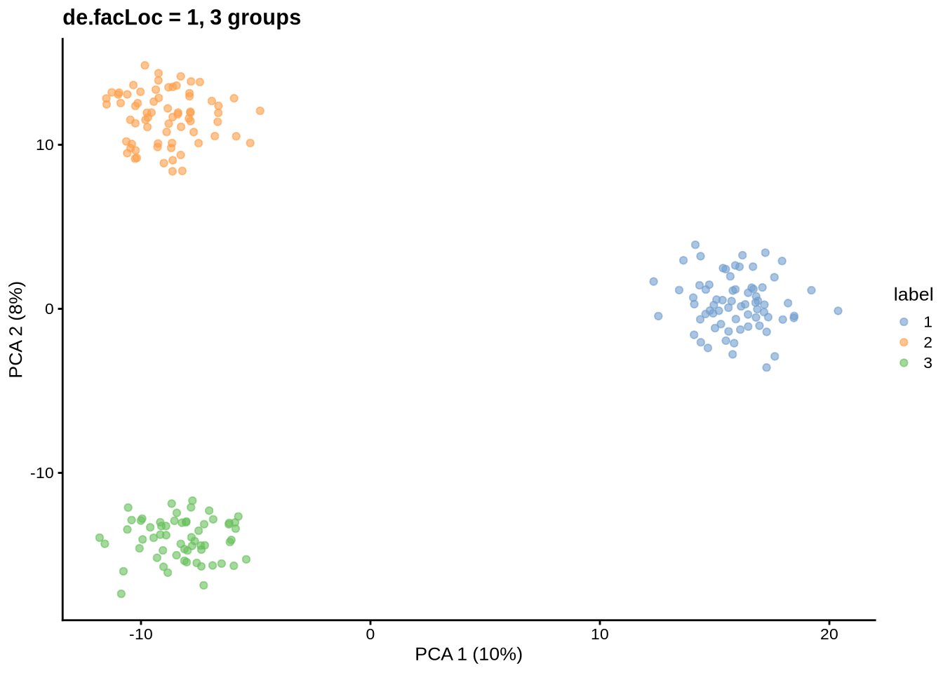
params@de.facLoc <- 2
sce <- splatSimulateGroups(params)
Getting parameters...Creating simulation object...Simulating library sizes...Simulating gene means...Simulating group DE...Simulating cell means...Simulating BCV...Warning in splatSimBCVMeans(sim, params): 'bcv.df' is infinite. This parameter
will be ignored.Simulating counts...Simulating dropout (if needed)...Sparsifying assays...Automatically converting to sparse matrices, threshold = 0.95Skipping 'BatchCellMeans': estimated sparse size 1.5 * dense matrixSkipping 'BaseCellMeans': estimated sparse size 1.5 * dense matrixSkipping 'BCV': estimated sparse size 1.5 * dense matrixSkipping 'CellMeans': estimated sparse size 1.5 * dense matrixSkipping 'TrueCounts': estimated sparse size 2.65 * dense matrixSkipping 'counts': estimated sparse size 2.65 * dense matrixDone!plot_pca(sce) + ggtitle("de.facLoc = 2, 3 groups")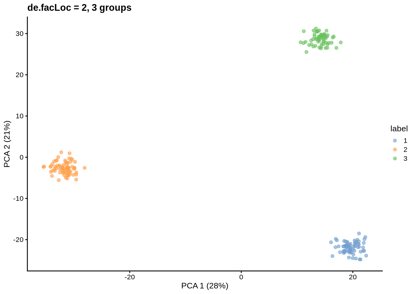
params@de.facLoc <- 0.1Differential expression scale
By default 0.4
params@de.facScale <- 0.6
sce <- splatSimulateGroups(params)
Getting parameters...Creating simulation object...Simulating library sizes...Simulating gene means...Simulating group DE...Simulating cell means...Simulating BCV...Warning in splatSimBCVMeans(sim, params): 'bcv.df' is infinite. This parameter
will be ignored.Simulating counts...Simulating dropout (if needed)...Sparsifying assays...Automatically converting to sparse matrices, threshold = 0.95Skipping 'BatchCellMeans': estimated sparse size 1.5 * dense matrixSkipping 'BaseCellMeans': estimated sparse size 1.5 * dense matrixSkipping 'BCV': estimated sparse size 1.5 * dense matrixSkipping 'CellMeans': estimated sparse size 1.5 * dense matrixSkipping 'TrueCounts': estimated sparse size 2.7 * dense matrixSkipping 'counts': estimated sparse size 2.7 * dense matrixDone!plot_pca(sce) + ggtitle("de.facScale = 0.6, 3 groups")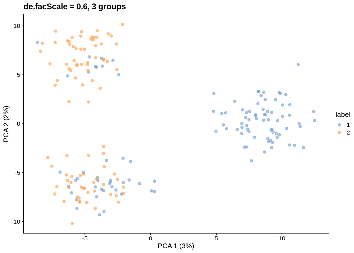
params@de.facScale <- 0.8
sce <- splatSimulateGroups(params)
Getting parameters...Creating simulation object...Simulating library sizes...Simulating gene means...Simulating group DE...Simulating cell means...Simulating BCV...Warning in splatSimBCVMeans(sim, params): 'bcv.df' is infinite. This parameter
will be ignored.Simulating counts...Simulating dropout (if needed)...Sparsifying assays...Automatically converting to sparse matrices, threshold = 0.95Skipping 'BatchCellMeans': estimated sparse size 1.5 * dense matrixSkipping 'BaseCellMeans': estimated sparse size 1.5 * dense matrixSkipping 'BCV': estimated sparse size 1.5 * dense matrixSkipping 'CellMeans': estimated sparse size 1.5 * dense matrixSkipping 'TrueCounts': estimated sparse size 2.7 * dense matrixSkipping 'counts': estimated sparse size 2.7 * dense matrixDone!plot_pca(sce) + ggtitle("de.facScale = 0.8, 3 groups")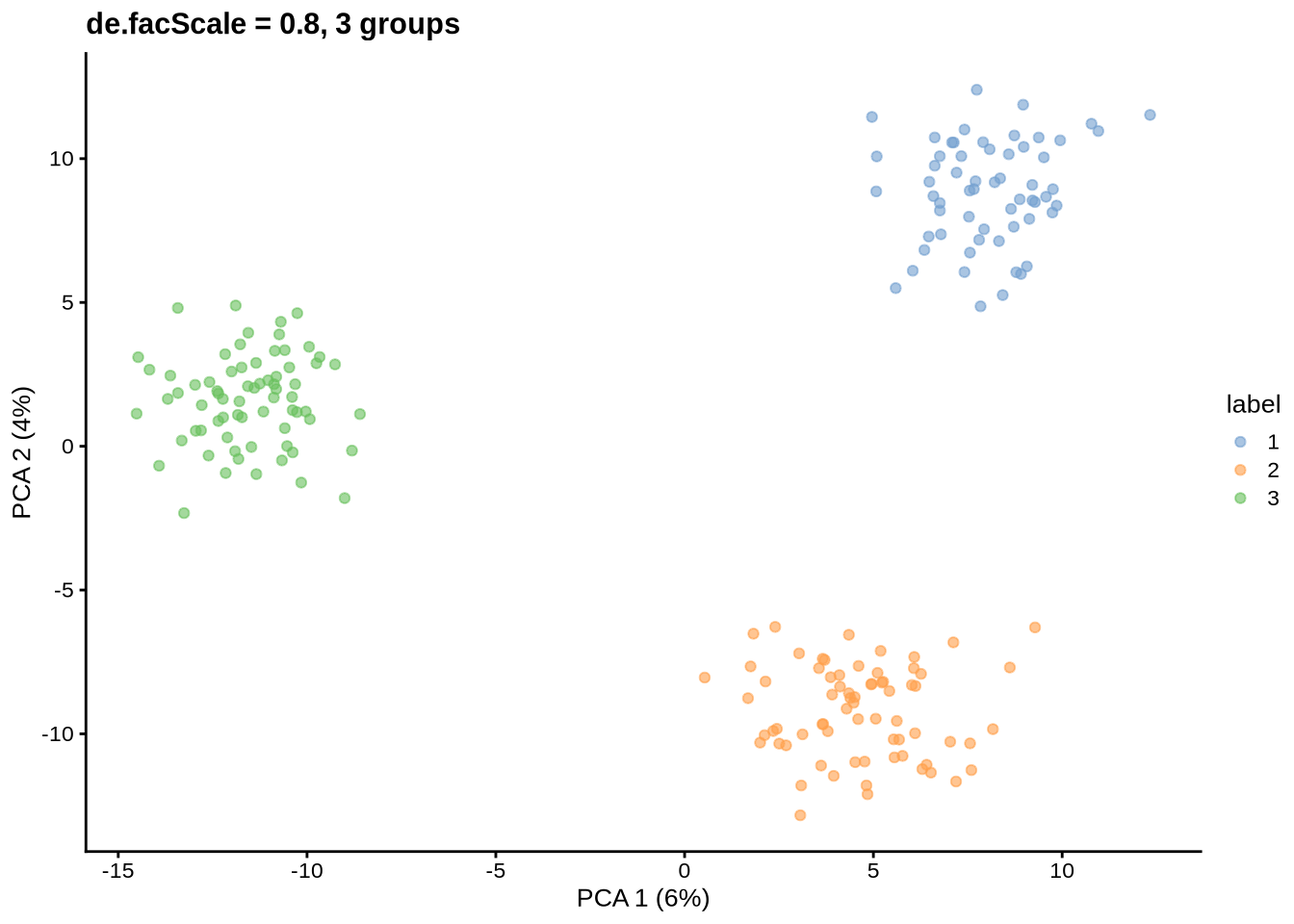
params@de.facScale <- 1.2
sce <- splatSimulateGroups(params)
Getting parameters...Creating simulation object...Simulating library sizes...Simulating gene means...Simulating group DE...Simulating cell means...Simulating BCV...Warning in splatSimBCVMeans(sim, params): 'bcv.df' is infinite. This parameter
will be ignored.Simulating counts...Simulating dropout (if needed)...Sparsifying assays...Automatically converting to sparse matrices, threshold = 0.95Skipping 'BatchCellMeans': estimated sparse size 1.5 * dense matrixSkipping 'BaseCellMeans': estimated sparse size 1.5 * dense matrixSkipping 'BCV': estimated sparse size 1.5 * dense matrixSkipping 'CellMeans': estimated sparse size 1.5 * dense matrixSkipping 'TrueCounts': estimated sparse size 2.69 * dense matrixSkipping 'counts': estimated sparse size 2.69 * dense matrixDone!plot_pca(sce) + ggtitle("de.facScale = 1.2, 3 groups")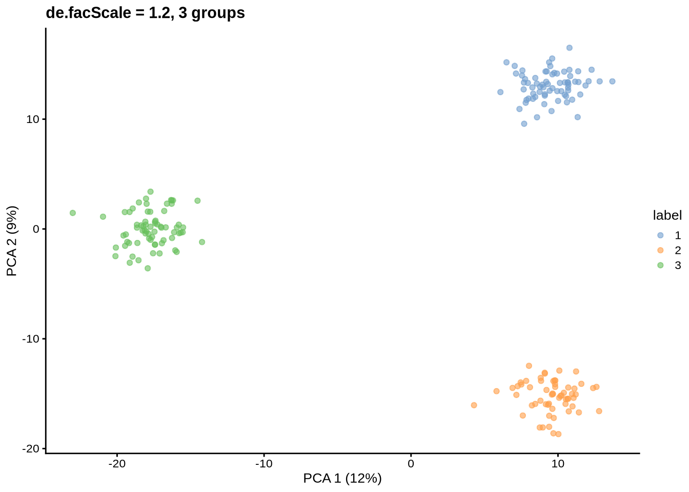
params@de.facScale <- 2
sce <- splatSimulateGroups(params)
Getting parameters...Creating simulation object...Simulating library sizes...Simulating gene means...Simulating group DE...Simulating cell means...Simulating BCV...Warning in splatSimBCVMeans(sim, params): 'bcv.df' is infinite. This parameter
will be ignored.Simulating counts...Simulating dropout (if needed)...Sparsifying assays...Automatically converting to sparse matrices, threshold = 0.95Skipping 'BatchCellMeans': estimated sparse size 1.5 * dense matrixSkipping 'BaseCellMeans': estimated sparse size 1.5 * dense matrixSkipping 'BCV': estimated sparse size 1.5 * dense matrixSkipping 'CellMeans': estimated sparse size 1.5 * dense matrixSkipping 'TrueCounts': estimated sparse size 2.65 * dense matrixSkipping 'counts': estimated sparse size 2.65 * dense matrixDone!plot_pca(sce) + ggtitle("de.facScale = 2, 3 groups")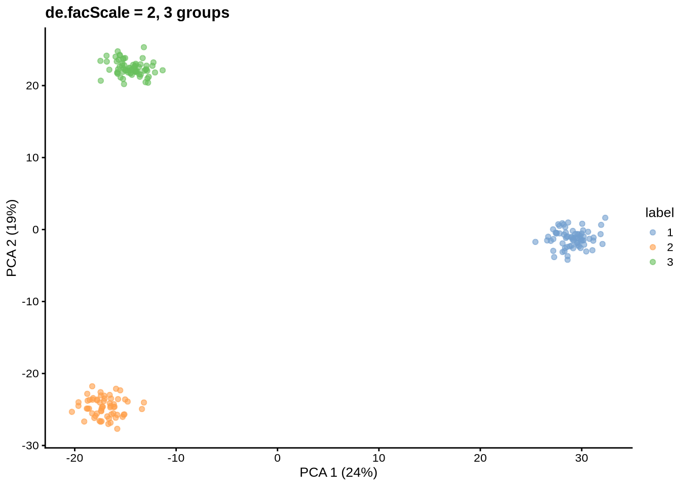
params@de.facScale <- 0.4library(ggplot2)
library(SingleCellExperiment)
library(scater)Standard simulation
standard_sim <- readRDS(here::here("data", "sim_data", "standard_sim_1-pbmc3k.rds"))plotPCA(standard_sim, colour_by = "Group")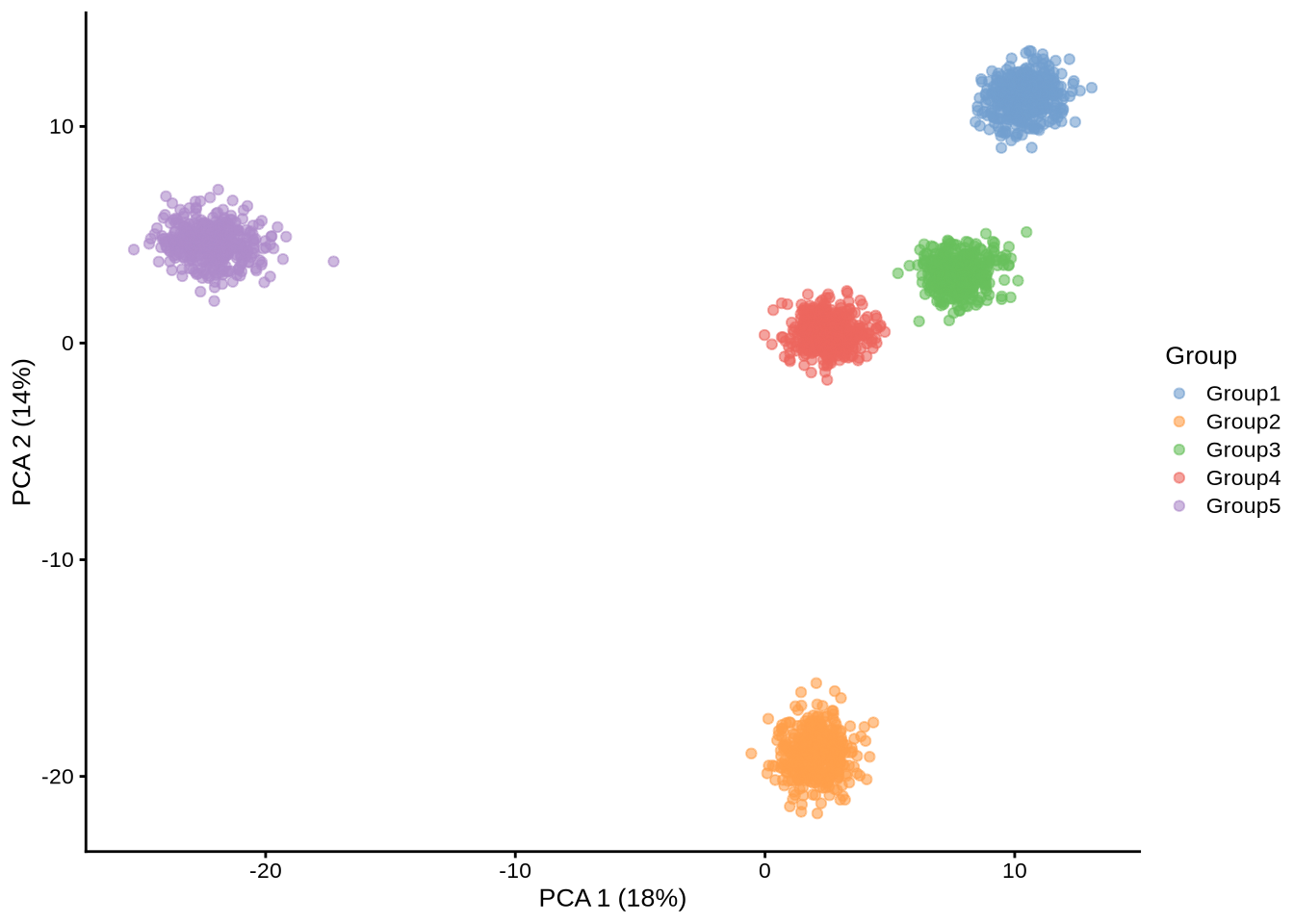
plotTSNE(standard_sim, colour_by = "Group")
# Don't use memory we don't absolutely have to.
rm(standard_sim)library(dplyr)
library(SingleCellExperiment)
library(tibble)
library(ggplot2)
library(scater)# config <- yaml::read_yaml(here::here("config.yaml"))
#
# umg_paths <- list.files(here::here(config$sim_data_folder), pattern = "^umg",
# full.names = TRUE)
# umgs <- lapply(umg_paths, readRDS)
#
# sim_names <- substr(basename(umg_paths), 5, nchar(basename(umg_paths)) - 4)
# mgs <- tibble(sim_name = sim_names, umg = umgs, sumg = sumgs)
#
# pars <- retrive_simulation_parameters() %>%
# # HACK!!!!!
# mutate(sim_name = paste0(sim_name, "-", data_id)) %>%
# left_join(mgs, by = "sim_name") %>%
# pivot_longer(cols = c(umg, sumg),
# names_to = "mg_type",
# values_to = "mgs") %>%
# filter(mg_type == "umg") %>%
# # Just select one method.
# filter(pars == "seurat_poisson") %>%
# filter(rep == 1)
#
# zeisel_mgs <- pars %>%
# filter(data_id == "zeisel") %>%
# pull(mgs) %>%
# pluck(1) %>%
# lapply(function(x) get_top_true_mgs(x, direction = "up")) %>%
# # Work with the first cluster.
# pluck(1) %>%
# as_tibble()
#
# pbmc3k_mgs <- pars %>%
# filter(data_id == "pbmc3k") %>%
# pull(mgs) %>%
# pluck(1) %>%
# lapply(function(x) get_top_true_mgs(x, direction = "up",
# sort_by_score = "mean_score")) %>%
# # Work with the first cluster.
# pluck(1) %>%
# as_tibble()
#
# lawlor_mgs <- pars %>%
# filter(data_id == "lawlor") %>%
# pull(mgs) %>%
# pluck(1) %>%
# lapply(function(x) get_top_true_mgs(x, direction = "up")) %>%
# # Work with the first cluster.
# pluck(1) %>%
# as_tibble()sim_data_folder <- here::here("data", "sim_data")
pbmc3k_1 <- readRDS(file.path(sim_data_folder, "standard_sim_1-pbmc3k.rds"))
zeisel_1 <- readRDS(file.path(sim_data_folder, "standard_sim_1-zeisel.rds"))
lawlor_1 <- readRDS(file.path(sim_data_folder, "standard_sim_1-lawlor.rds"))#plotExpression(pbmc3k_1, features = pbmc3k_mgs$gene[1:20], x = "label")
rowData(pbmc3k_1) %>%
as_tibble() %>%
filter(Gene == "Gene931")# A tibble: 1 × 9
Gene BaseGeneMean OutlierFactor GeneMean DEFacGroup1 DEFacGroup2 DEFacGroup3
<chr> <dbl> <dbl> <dbl> <dbl> <dbl> <dbl>
1 Gene9… 0.153 1 0.153 1 1 1
# … with 2 more variables: DEFacGroup4 <dbl>, DEFacGroup5 <dbl>rowData(pbmc3k_1) %>%
as_tibble() %>%
filter(Gene == "Gene1080")# A tibble: 1 × 9
Gene BaseGeneMean OutlierFactor GeneMean DEFacGroup1 DEFacGroup2 DEFacGroup3
<chr> <dbl> <dbl> <dbl> <dbl> <dbl> <dbl>
1 Gene1… 0.0873 1 0.0873 31.5 1 1
# … with 2 more variables: DEFacGroup4 <dbl>, DEFacGroup5 <dbl>rowData(pbmc3k_1) %>%
as_tibble() %>%
filter(OutlierFactor > 1 & DEFacGroup1 < 1)# A tibble: 0 × 9
# … with 9 variables: Gene <chr>, BaseGeneMean <dbl>, OutlierFactor <dbl>,
# GeneMean <dbl>, DEFacGroup1 <dbl>, DEFacGroup2 <dbl>, DEFacGroup3 <dbl>,
# DEFacGroup4 <dbl>, DEFacGroup5 <dbl>plotExpression(pbmc3k_1, features = c("Gene370", "Gene1980"), x = "label")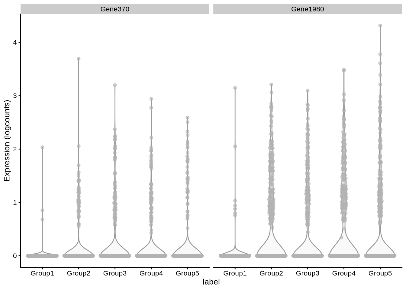
readRDS(here::here("results", "sim_data", "standard_sim_1-pbmc3k-seurat_wilcox.rds"))$time
[1] 13.776
$result
# A tibble: 2,485 × 7
p_value p_value_adj cluster log_fc gene raw_statistic scaled_statistic
<dbl> <dbl> <fct> <dbl> <chr> <dbl> <dbl>
1 4.54e-272 9.05e-269 Group1 3.60 Gene1080 0 0
2 3.28e-271 6.54e-268 Group1 3.67 Gene319 0 0
3 9.54e-271 1.90e-267 Group1 3.41 Gene376 0 0
4 1.17e-265 2.33e-262 Group1 3.47 Gene1904 0 0
5 5.14e-265 1.02e-261 Group1 4.15 Gene1637 0 0
6 4.75e-263 9.47e-260 Group1 4.32 Gene37 0 0
7 1.26e-262 2.50e-259 Group1 3.19 Gene1916 0 0
8 9.40e-261 1.87e-257 Group1 3.96 Gene823 0 0
9 1.22e-260 2.42e-257 Group1 4.41 Gene1228 0 0
10 1.40e-260 2.78e-257 Group1 3.64 Gene1604 0 0
# … with 2,475 more rows
$raw_result
# A tibble: 2,485 × 7
p_val avg_log2FC pct.1 pct.2 p_val_adj cluster gene
<dbl> <dbl> <dbl> <dbl> <dbl> <fct> <chr>
1 4.54e-272 3.60 0.926 0.109 9.05e-269 Group1 Gene1080
2 3.28e-271 3.67 0.926 0.119 6.54e-268 Group1 Gene319
3 9.54e-271 3.41 0.903 0.094 1.90e-267 Group1 Gene376
4 1.17e-265 3.47 0.908 0.104 2.33e-262 Group1 Gene1904
5 5.14e-265 4.15 0.957 0.154 1.02e-261 Group1 Gene1637
6 4.75e-263 4.32 0.974 0.183 9.47e-260 Group1 Gene37
7 1.26e-262 3.19 0.903 0.108 2.50e-259 Group1 Gene1916
8 9.40e-261 3.96 0.949 0.153 1.87e-257 Group1 Gene823
9 1.22e-260 4.41 0.967 0.179 2.42e-257 Group1 Gene1228
10 1.40e-260 3.64 0.959 0.162 2.78e-257 Group1 Gene1604
# … with 2,475 more rows
$pars
$pars$method
[1] "seurat"
$pars$test.use
[1] "wilcox"
$pars$file_name
[1] "seurat_wilcox"seurat_t <- readRDS(
here::here("results", "sim_data", "standard_sim_1-pbmc3k-seurat_t.rds")
)
seurat_t %>%
pluck("result") %>%
filter(log_fc < 0)# A tibble: 1,793 × 7
p_value p_value_adj cluster log_fc gene raw_statistic scaled_statistic
<dbl> <dbl> <fct> <dbl> <chr> <dbl> <dbl>
1 1.94e-223 3.86e-220 Group1 -5.91 Gene1623 0 0
2 4.06e-197 8.09e-194 Group1 -1.87 Gene1435 0 0
3 1.16e-185 2.31e-182 Group1 -4.35 Gene1638 0 0
4 5.48e-181 1.09e-177 Group1 -2.14 Gene71 0 0
5 2.23e-180 4.45e-177 Group1 -1.93 Gene790 0 0
6 2.90e-174 5.79e-171 Group1 -3.85 Gene1011 0 0
7 5.47e-172 1.09e-168 Group1 -3.69 Gene548 0 0
8 7.89e-171 1.57e-167 Group1 -2.09 Gene76 0 0
9 6.43e-162 1.28e-158 Group1 -4.03 Gene1596 0 0
10 8.51e-162 1.70e-158 Group1 -1.81 Gene60 0 0
# … with 1,783 more rowsplotExpression(pbmc3k_1, x = "label", features = "Gene1980")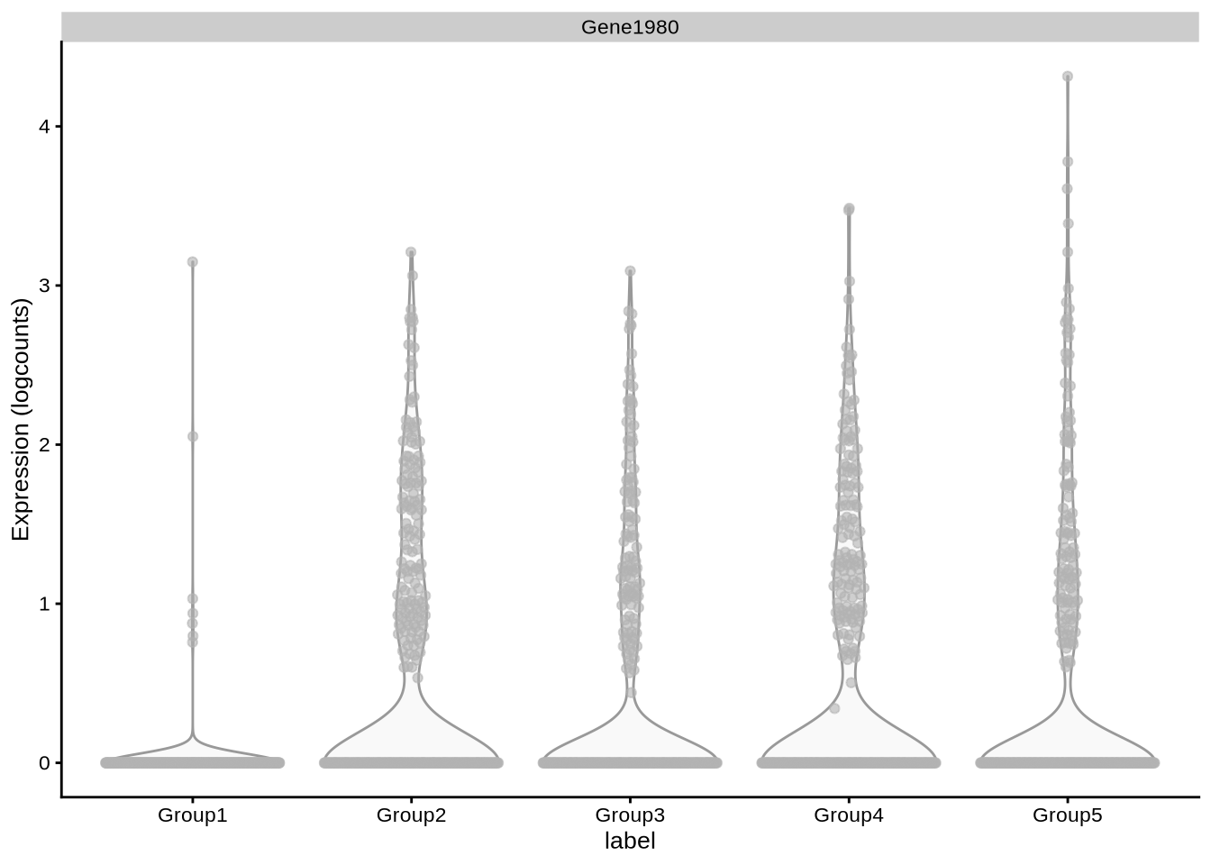
rowSums(counts(pbmc3k_1[281, ]))Gene282
52 # plotExpression(pbmc3k_1, features = pbmc3k_mgs$gene[1:10], x = "label")
# plotExpression(pbmc3k_1, features = pbmc3k_mgs$gene[50:60], x = "label")
# plotExpression(pbmc3k_1, features = pbmc3k_mgs$gene[100:110], x = "label")# means_1 <- rowMeans(counts(pbmc3k_1[pbmc3k_mgs$gene, pbmc3k_1$label == "Group1"]))
# means_2 <- rowMeans(counts(pbmc3k_1[pbmc3k_mgs$gene, pbmc3k_1$label != "Group1"]))
# log_fcs <- log(means_1 / means_2)
#
# tibble(rank = 1:length(log_fcs), log_fc = log_fcs) %>%
# ggplot(aes(x = rank, y = log_fc)) +
# geom_point(colour = "seagreen") +
# labs(
# x = "True marker gene rank",
# y = "Two sample log fold change"
# ) +
# theme_bw()# plotExpression(zeisel_1, features = zeisel_mgs$gene[1:10], x = "label")
# plotExpression(zeisel_1, features = zeisel_mgs$gene[50:60], x = "label")
# plotExpression(zeisel_1, features = zeisel_mgs$gene[100:110], x = "label")# plotExpression(lawlor_1, features = lawlor_mgs$gene[1:5], x = "label")
# plotExpression(lawlor_1, features = lawlor_mgs$gene[50:55], x = "label")
# plotExpression(lawlor_1, features = lawlor_mgs$gene[100:105], x = "label")pbmc3k <- readRDS(here::here("data", "real_data", "pbmc3k.rds"))
calculate_mean_diff <- function(sce, cluster_label) {
counts <- counts(sce)
x <- as.numeric(colLabels(sce) == cluster_label)
n_genes <- nrow(sce)
out <- numeric(n_genes)
for (i in seq_len(n_genes)) {
y <- counts[i, ]
y_1 <- y[x == 0]
y_2 <- y[x == 1]
out[[i]] <- mean(y_1) - mean(y_2)
}
out
}
pbmc3k_mean_diff <- calculate_mean_diff(pbmc3k, "Group1")
data.frame(mean_diff = pbmc3k_mean_diff) %>%
ggplot(aes(mean_diff)) +
geom_histogram(bins = 30)Warning: Removed 2000 rows containing non-finite values (stat_bin).
devtools::session_info()─ Session info ──────────────────────────────────────────────────────────────
hash: clinking beer mugs, dress, weary face
setting value
version R version 4.1.2 (2021-11-01)
os Red Hat Enterprise Linux 9.2 (Plow)
system x86_64, linux-gnu
ui X11
language (EN)
collate en_AU.UTF-8
ctype en_AU.UTF-8
tz Australia/Melbourne
date 2024-01-01
pandoc 2.18 @ /apps/easybuild-2022/easybuild/software/MPI/GCC/11.3.0/OpenMPI/4.1.4/RStudio-Server/2022.07.2+576-Java-11-R-4.1.2/bin/pandoc/ (via rmarkdown)
─ Packages ───────────────────────────────────────────────────────────────────
package * version date (UTC) lib source
assertthat 0.2.1 2019-03-21 [2] CRAN (R 4.1.2)
backports 1.3.0 2021-10-27 [2] CRAN (R 4.1.2)
beachmat 2.10.0 2021-10-26 [1] Bioconductor
beeswarm 0.4.0 2021-06-01 [2] CRAN (R 4.1.2)
Biobase * 2.54.0 2021-10-26 [1] Bioconductor
BiocGenerics * 0.40.0 2021-10-26 [1] Bioconductor
BiocNeighbors 1.12.0 2021-10-26 [1] Bioconductor
BiocParallel 1.28.3 2021-12-09 [1] Bioconductor
BiocSingular 1.10.0 2021-10-26 [1] Bioconductor
bitops 1.0-7 2021-04-24 [2] CRAN (R 4.1.2)
bluster 1.4.0 2021-10-26 [1] Bioconductor
bslib 0.3.1 2021-10-06 [1] CRAN (R 4.1.0)
cachem 1.0.6 2021-08-19 [1] CRAN (R 4.1.0)
callr 3.7.0 2021-04-20 [2] CRAN (R 4.1.2)
checkmate 2.0.0 2020-02-06 [2] CRAN (R 4.1.2)
cli 3.6.1 2023-03-23 [1] CRAN (R 4.1.0)
cluster 2.1.2 2021-04-17 [2] CRAN (R 4.1.2)
colorspace 2.1-0 2023-01-23 [1] CRAN (R 4.1.0)
cowplot 1.1.1 2020-12-30 [2] CRAN (R 4.1.2)
crayon 1.5.1 2022-03-26 [1] CRAN (R 4.1.0)
DBI 1.1.2 2021-12-20 [1] CRAN (R 4.1.0)
DelayedArray 0.20.0 2021-10-26 [1] Bioconductor
DelayedMatrixStats 1.16.0 2021-10-26 [1] Bioconductor
desc 1.4.0 2021-09-28 [2] CRAN (R 4.1.2)
devtools 2.4.2 2021-06-07 [2] CRAN (R 4.1.2)
digest 0.6.29 2021-12-01 [1] CRAN (R 4.1.0)
dplyr * 1.0.9 2022-04-28 [1] CRAN (R 4.1.0)
dqrng 0.3.0 2021-05-01 [1] CRAN (R 4.1.0)
edgeR 3.36.0 2021-10-26 [1] Bioconductor
ellipsis 0.3.2 2021-04-29 [2] CRAN (R 4.1.2)
evaluate 0.14 2019-05-28 [2] CRAN (R 4.1.2)
fansi 1.0.4 2023-01-22 [1] CRAN (R 4.1.0)
farver 2.1.1 2022-07-06 [1] CRAN (R 4.1.0)
fastmap 1.1.0 2021-01-25 [2] CRAN (R 4.1.2)
fitdistrplus 1.1-8 2022-03-10 [1] CRAN (R 4.1.0)
fs 1.5.2 2021-12-08 [1] CRAN (R 4.1.0)
generics 0.1.3 2022-07-05 [1] CRAN (R 4.1.0)
GenomeInfoDb * 1.30.0 2021-10-26 [1] Bioconductor
GenomeInfoDbData 1.2.7 2021-12-03 [1] Bioconductor
GenomicRanges * 1.46.1 2021-11-18 [1] Bioconductor
ggbeeswarm 0.6.0 2017-08-07 [2] CRAN (R 4.1.2)
ggplot2 * 3.3.6 2022-05-03 [1] CRAN (R 4.1.0)
ggrepel 0.9.1 2021-01-15 [2] CRAN (R 4.1.2)
git2r 0.28.0 2021-01-10 [2] CRAN (R 4.1.2)
glue 1.6.0 2021-12-17 [1] CRAN (R 4.1.0)
gridExtra 2.3 2017-09-09 [2] CRAN (R 4.1.2)
gtable 0.3.0 2019-03-25 [2] CRAN (R 4.1.2)
here 1.0.1 2020-12-13 [1] CRAN (R 4.1.0)
highr 0.9 2021-04-16 [2] CRAN (R 4.1.2)
htmltools 0.5.2 2021-08-25 [1] CRAN (R 4.1.0)
httpuv 1.6.5 2022-01-05 [1] CRAN (R 4.1.0)
igraph 1.3.2 2022-06-13 [1] CRAN (R 4.1.0)
IRanges * 2.28.0 2021-10-26 [1] Bioconductor
irlba 2.3.5 2021-12-06 [1] CRAN (R 4.1.0)
jquerylib 0.1.4 2021-04-26 [2] CRAN (R 4.1.2)
jsonlite 1.8.0 2022-02-22 [1] CRAN (R 4.1.0)
knitr 1.36 2021-09-29 [1] CRAN (R 4.1.0)
labeling 0.4.2 2020-10-20 [2] CRAN (R 4.1.2)
later 1.3.0 2021-08-18 [1] CRAN (R 4.1.0)
lattice 0.20-45 2021-09-22 [2] CRAN (R 4.1.2)
lifecycle 1.0.1 2021-09-24 [1] CRAN (R 4.1.0)
limma 3.50.0 2021-10-26 [1] Bioconductor
locfit 1.5-9.4 2020-03-25 [2] CRAN (R 4.1.2)
magrittr 2.0.3 2022-03-30 [1] CRAN (R 4.1.0)
MASS 7.3-54 2021-05-03 [2] CRAN (R 4.1.2)
Matrix 1.3-4 2021-06-01 [2] CRAN (R 4.1.2)
MatrixGenerics * 1.6.0 2021-10-26 [1] Bioconductor
matrixStats * 0.62.0 2022-04-19 [1] CRAN (R 4.1.0)
memoise 2.0.1 2021-11-26 [1] CRAN (R 4.1.0)
metapod 1.2.0 2021-10-26 [1] Bioconductor
munsell 0.5.0 2018-06-12 [2] CRAN (R 4.1.2)
pillar 1.7.0 2022-02-01 [1] CRAN (R 4.1.0)
pkgbuild 1.2.0 2020-12-15 [2] CRAN (R 4.1.2)
pkgconfig 2.0.3 2019-09-22 [2] CRAN (R 4.1.2)
pkgload 1.2.3 2021-10-13 [2] CRAN (R 4.1.2)
prettyunits 1.1.1 2020-01-24 [2] CRAN (R 4.1.2)
processx 3.5.2 2021-04-30 [2] CRAN (R 4.1.2)
promises 1.2.0.1 2021-02-11 [2] CRAN (R 4.1.2)
ps 1.7.1 2022-06-18 [1] CRAN (R 4.1.0)
purrr * 0.3.4 2020-04-17 [2] CRAN (R 4.1.2)
R6 2.5.1 2021-08-19 [1] CRAN (R 4.1.0)
Rcpp 1.0.8.3 2022-03-17 [1] CRAN (R 4.1.0)
RCurl 1.98-1.5 2021-09-17 [1] CRAN (R 4.1.0)
remotes 2.4.2 2021-11-30 [1] CRAN (R 4.1.0)
rlang 1.0.3 2022-06-27 [1] CRAN (R 4.1.0)
rmarkdown 2.14 2022-04-25 [1] CRAN (R 4.1.0)
rprojroot 2.0.3 2022-04-02 [1] CRAN (R 4.1.0)
rstudioapi 0.14 2022-08-22 [1] CRAN (R 4.1.0)
rsvd 1.0.5 2021-04-16 [1] CRAN (R 4.1.0)
S4Vectors * 0.32.3 2021-11-21 [1] Bioconductor
sass 0.4.1 2022-03-23 [1] CRAN (R 4.1.0)
ScaledMatrix 1.2.0 2021-10-26 [1] Bioconductor
scales 1.2.1 2022-08-20 [1] CRAN (R 4.1.0)
scater * 1.22.0 2021-10-26 [1] Bioconductor
scran * 1.22.1 2021-11-14 [1] Bioconductor
scuttle * 1.4.0 2021-10-26 [1] Bioconductor
sessioninfo 1.2.0 2021-10-31 [2] CRAN (R 4.1.2)
SingleCellExperiment * 1.16.0 2021-10-26 [1] Bioconductor
sparseMatrixStats * 1.6.0 2021-10-26 [1] Bioconductor
splatter * 1.18.1 2021-11-02 [1] Bioconductor
statmod 1.4.36 2021-05-10 [2] CRAN (R 4.1.2)
stringi 1.7.6 2021-11-29 [1] CRAN (R 4.1.0)
stringr 1.4.0 2019-02-10 [2] CRAN (R 4.1.2)
SummarizedExperiment * 1.24.0 2021-10-26 [1] Bioconductor
survival 3.2-13 2021-08-24 [2] CRAN (R 4.1.2)
testthat 3.1.0 2021-10-04 [2] CRAN (R 4.1.2)
tibble * 3.1.7 2022-05-03 [1] CRAN (R 4.1.0)
tidyr 1.2.0 2022-02-01 [1] CRAN (R 4.1.0)
tidyselect 1.1.2 2022-02-21 [1] CRAN (R 4.1.0)
usethis 2.1.3 2021-10-27 [2] CRAN (R 4.1.2)
utf8 1.2.3 2023-01-31 [1] CRAN (R 4.1.0)
vctrs 0.4.1 2022-04-13 [1] CRAN (R 4.1.0)
vipor 0.4.5 2017-03-22 [2] CRAN (R 4.1.2)
viridis 0.6.2 2021-10-13 [1] CRAN (R 4.1.0)
viridisLite 0.4.2 2023-05-02 [1] CRAN (R 4.1.0)
whisker 0.4 2019-08-28 [2] CRAN (R 4.1.2)
withr 2.5.0 2022-03-03 [1] CRAN (R 4.1.0)
workflowr 1.7.0 2021-12-21 [1] CRAN (R 4.1.0)
xfun 0.31 2022-05-10 [1] CRAN (R 4.1.0)
XVector 0.34.0 2021-10-26 [1] Bioconductor
yaml 2.3.5 2022-02-21 [1] CRAN (R 4.1.0)
zlibbioc 1.40.0 2021-10-26 [1] Bioconductor
[1] /home/jpullin/R/x86_64-pc-linux-gnu-library/4.1
[2] /apps/easybuild-2022/easybuild/software/MPI/GCC/11.3.0/OpenMPI/4.1.4/R/4.1.2/lib64/R/library
──────────────────────────────────────────────────────────────────────────────