Simulation validation analysis
Last updated: 2024-01-01
Checks: 7 0
Knit directory:
mage_2020_marker-gene-benchmarking/
This reproducible R Markdown analysis was created with workflowr (version 1.7.0). The Checks tab describes the reproducibility checks that were applied when the results were created. The Past versions tab lists the development history.
Great! Since the R Markdown file has been committed to the Git repository, you know the exact version of the code that produced these results.
Great job! The global environment was empty. Objects defined in the global environment can affect the analysis in your R Markdown file in unknown ways. For reproduciblity it’s best to always run the code in an empty environment.
The command set.seed(20190102) was run prior to running
the code in the R Markdown file. Setting a seed ensures that any results
that rely on randomness, e.g. subsampling or permutations, are
reproducible.
Great job! Recording the operating system, R version, and package versions is critical for reproducibility.
Nice! There were no cached chunks for this analysis, so you can be confident that you successfully produced the results during this run.
Great job! Using relative paths to the files within your workflowr project makes it easier to run your code on other machines.
Great! You are using Git for version control. Tracking code development and connecting the code version to the results is critical for reproducibility.
The results in this page were generated with repository version 2632193. See the Past versions tab to see a history of the changes made to the R Markdown and HTML files.
Note that you need to be careful to ensure that all relevant files for
the analysis have been committed to Git prior to generating the results
(you can use wflow_publish or
wflow_git_commit). workflowr only checks the R Markdown
file, but you know if there are other scripts or data files that it
depends on. Below is the status of the Git repository when the results
were generated:
Ignored files:
    Ignored:    .Renviron
    Ignored:    .Rhistory
    Ignored:    .Rproj.user/
    Ignored:    .snakemake/
    Ignored:    NSForest/.Rhistory
    Ignored:    NSForest/NS-Forest_v3_Extended_Binary_Markers_Supplmental.csv
    Ignored:    NSForest/NS-Forest_v3_Full_Results.csv
    Ignored:    NSForest/NSForest3_medianValues.csv
    Ignored:    NSForest/NSForest_v3_Final_Result.csv
    Ignored:    NSForest/__pycache__/
    Ignored:    NSForest/data/
    Ignored:    RankCorr/picturedRocks/__pycache__/
    Ignored:    benchmarks/
    Ignored:    config/
    Ignored:    data/cellmarker/
    Ignored:    data/downloaded_data/
    Ignored:    data/expert_annotations/
    Ignored:    data/expert_mgs/
    Ignored:    data/raw_data/
    Ignored:    data/real_data/
    Ignored:    data/sim_data/
    Ignored:    data/sim_mgs/
    Ignored:    data/special_real_data/
    Ignored:    figures/
    Ignored:    logs/
    Ignored:    results/
    Ignored:    weights/

Unstaged changes:
    Deleted:    analysis/expert-mgs-direction.Rmd
    Modified:   smash-fork
Note that any generated files, e.g. HTML, png, CSS, etc., are not included in this status report because it is ok for generated content to have uncommitted changes.
These are the previous versions of the repository in which changes were
made to the R Markdown
(analysis/simulation-validation-analysis.Rmd) and HTML
(public/simulation-validation-analysis.html) files. If
you’ve configured a remote Git repository (see
?wflow_git_remote), click on the hyperlinks in the table
below to view the files as they were in that past version.
| File | Version | Author | Date | Message |
|---|---|---|---|---|
| html | fcecf65 | Jeffrey Pullin | 2022-09-09 | Build site. |
| Rmd | 0c2eafc | Jeffrey Pullin | 2022-09-09 | Update website |
| html | af96b34 | Jeffrey Pullin | 2022-08-30 | Build site. |
| Rmd | a2056d7 | Jeffrey Pullin | 2022-08-29 | Add more simulation validation analysis |
| html | 0e47874 | Jeffrey Pullin | 2022-05-04 | Build site. |
| html | 8b989e1 | Jeffrey Pullin | 2022-05-02 | Build site. |
| html | 0548273 | Jeffrey Pullin | 2022-05-02 | Build site. |
| Rmd | 50bca7c | Jeffrey Pullin | 2022-05-02 | workflowr::wflow_publish(all = TRUE, republish = TRUE) |
| html | 50bca7c | Jeffrey Pullin | 2022-05-02 | workflowr::wflow_publish(all = TRUE, republish = TRUE) |
| html | 5cc008f | Jeffrey Pullin | 2022-02-09 | Build site. |
| Rmd | d1aca16 | Jeffrey Pullin | 2022-02-09 | Refresh website |
| Rmd | aca9ad2 | Jeffrey Pullin | 2021-11-29 | Various changes made in the last days before thesis submission |
library(SingleCellExperiment)
library(dplyr)
library(ggplot2)
library(patchwork)
library(scater)
library(purrr)
library(tidyr)

source(here::here("code", "analysis-utils.R"))
source(here::here("code", "run-utils.R"))
Load data
pbmc3k_sim <- readRDS(
  here::here("data", "sim_data", "standard_sim_1-pbmc3k.rds")
)

lawlor_sim <- readRDS(
  here::here("data", "sim_data", "standard_sim_1-lawlor.rds")
)

zeisel_sim <- readRDS(
  here::here("data", "sim_data", "standard_sim_1-zeisel.rds")
)

endothelial_sim <- readRDS(
  here::here("data", "sim_data", "standard_sim_1-endothelial.rds")
)
pbmc3k <- readRDS(
here::here("data", "real_data", "pbmc3k.rds")
)
lawlor <- readRDS(
here::here("data", "real_data", "lawlor.rds")
)
zeisel <- readRDS(
here::here("data", "real_data", "zeisel.rds")
)
endothelial <- readRDS(
here::here("data", "real_data", "endothelial.rds")
)pbmc3k_mg_info <- readRDS(
here::here("data", "sim_mgs", "mg-standard_sim_1-pbmc3k.rds")
)
lawlor_mg_info <- readRDS(
here::here("data", "sim_mgs", "mg-standard_sim_1-lawlor.rds")
)
zeisel_mg_info <- readRDS(
here::here("data", "sim_mgs", "mg-standard_sim_1-zeisel.rds")
)
endothelial_mg_info <- readRDS(
here::here("data", "sim_mgs", "mg-standard_sim_1-endothelial.rds")
)pbmc3k_result <- readRDS(
here::here("results", "real_data", "pbmc3k-seurat_wilcox.rds")
)
lawlor_result <- readRDS(
here::here("results", "real_data", "lawlor-seurat_wilcox.rds")
)
zeisel_result <- readRDS(
here::here("results", "real_data", "zeisel-seurat_wilcox.rds")
)
endothelial_result <- readRDS(
here::here("results", "real_data", "endothelial-seurat_wilcox.rds")
)pbmc3k_sim_result <- readRDS(
here::here("results", "sim_data", "standard_sim_1-pbmc3k-seurat_wilcox.rds")
)
lawlor_sim_result <- readRDS(
here::here("results", "sim_data", "standard_sim_1-lawlor-seurat_wilcox.rds")
)
zeisel_sim_result <- readRDS(
here::here("results", "sim_data", "standard_sim_1-zeisel-seurat_wilcox.rds")
)
endothelial_sim_result <- readRDS(
here::here("results", "sim_data", "standard_sim_1-endothelial-seurat_wilcox.rds")
)pbmc3k_expert_mgs <- readRDS(
here::here("data", "expert_mgs", "pbmc3k_expert_mgs.rds")
)
lawlor_expert_mgs <- readRDS(
here::here("data", "expert_mgs", "lawlor_expert_mgs.rds")
)plot_specifc_mgs <- function(sce, mg_info, index = c(1, 10, 20, 30),
direction = "up", cluster_ind = 1) {
last_index <- index[length(index)]
top_mgs <- get_top_true_mgs(mg_info[[cluster_ind]], direction = "up",
n = last_index + 1)
specific_mgs <- top_mgs$gene[index]
plotExpression(sce, x = "label", features = specific_mgs)
}
plot_logfc_sim_mgs <- function(sce, mg_info, n = "all", direction = "up",
cluster_ind = 1) {
top_mgs <- get_top_true_mgs(mg_info[[cluster_ind]], direction = "up",
n = n)
if (n == "all") {
n <- nrow(top_mgs)
}
clusters <- rep(paste0("Group", cluster_ind), n)
log_fc <- calculate_log_fc(sce, top_mgs$gene, clusters)
plot_data <- tibble(
log_fc,
index = 1:n
)
ggplot(plot_data, aes(x = index, y = log_fc)) +
geom_point() +
geom_smooth(se = FALSE, formula = y ~ x, method = "loess") +
labs(
x = "Index",
y = "Log fold-change"
) +
theme_bw()
}
plot_logfc_real_mgs <- function(sce, result, cluster, n = 200, direction = "up") {
top_mgs <- result %>%
pluck("result") %>%
filter(cluster == !!cluster) %>%
get_top_sel_mgs(direction = "up", n = n)
clusters <- rep(cluster, n)
log_fc <- calculate_log_fc(sce, top_mgs$gene, clusters)
plot_data <- tibble(
log_fc,
index = 1:n
)
ggplot(plot_data, aes(x = index, y = log_fc)) +
geom_point() +
geom_smooth(se = FALSE, formula = y ~ x, method = "loess") +
labs(
x = "Index",
y = "Log fold-change"
) +
theme_bw()
}pbmc3k_top_sim_mgs <- pbmc3k_mg_info %>%
map(~ get_top_true_mgs(.x, n = 3, direction = "up")) %>%
imap(~ mutate(.x, cluster = .y)) %>%
bind_rows() %>%
mutate(cluster = paste0("Group", substr(cluster, 7, 7)))
pbmc3k_top_expert_mgs <- pbmc3k_expert_mgs %>%
unnest(expert_mgs) %>%
dplyr::rename(gene = expert_mgs)
pbmc3k_top_sim_logfcs <- calculate_log_fc(
pbmc3k_sim,
genes = pbmc3k_top_sim_mgs$gene,
clusters = pbmc3k_top_sim_mgs$cluster
)
pbmc3k_top_expert_logfcs <- calculate_log_fc(
pbmc3k,
genes = pbmc3k_top_expert_mgs$gene,
clusters = pbmc3k_top_expert_mgs$cluster
)
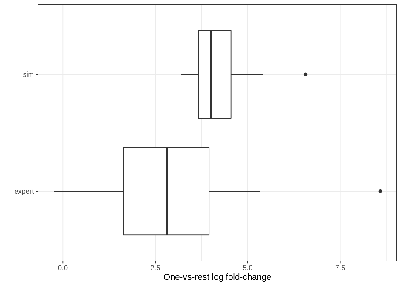
tibble(sim = pbmc3k_top_sim_logfcs, expert = pbmc3k_top_expert_logfcs) %>%
pivot_longer(cols = everything(), names_to = "type", values_to = "logfc") %>%
ggplot(aes(x = type, y = logfc)) +
geom_boxplot() +
coord_flip() +
theme_bw() +
labs(
x = "",
y = "One-vs-rest log fold-change"
)
lawlor_top_sim_mgs <- lawlor_mg_info %>%
map(~ get_top_true_mgs(.x, n = 1, direction = "up")) %>%
imap(~ mutate(.x, cluster = .y)) %>%
bind_rows() %>%
mutate(cluster = paste0("Group", substr(cluster, 7, 7)))
lawlor_top_expert_mgs <- lawlor_expert_mgs %>%
unnest(expert_mgs) %>%
rename(gene = expert_mgs)
lawlor_top_sim_logfcs <- calculate_log_fc(
lawlor_sim,
genes = lawlor_top_sim_mgs$gene,
clusters = lawlor_top_sim_mgs$cluster
)
lawlor_top_expert_logfcs <- calculate_log_fc(
lawlor,
genes = lawlor_top_expert_mgs$gene,
clusters = lawlor_top_expert_mgs$cluster
)
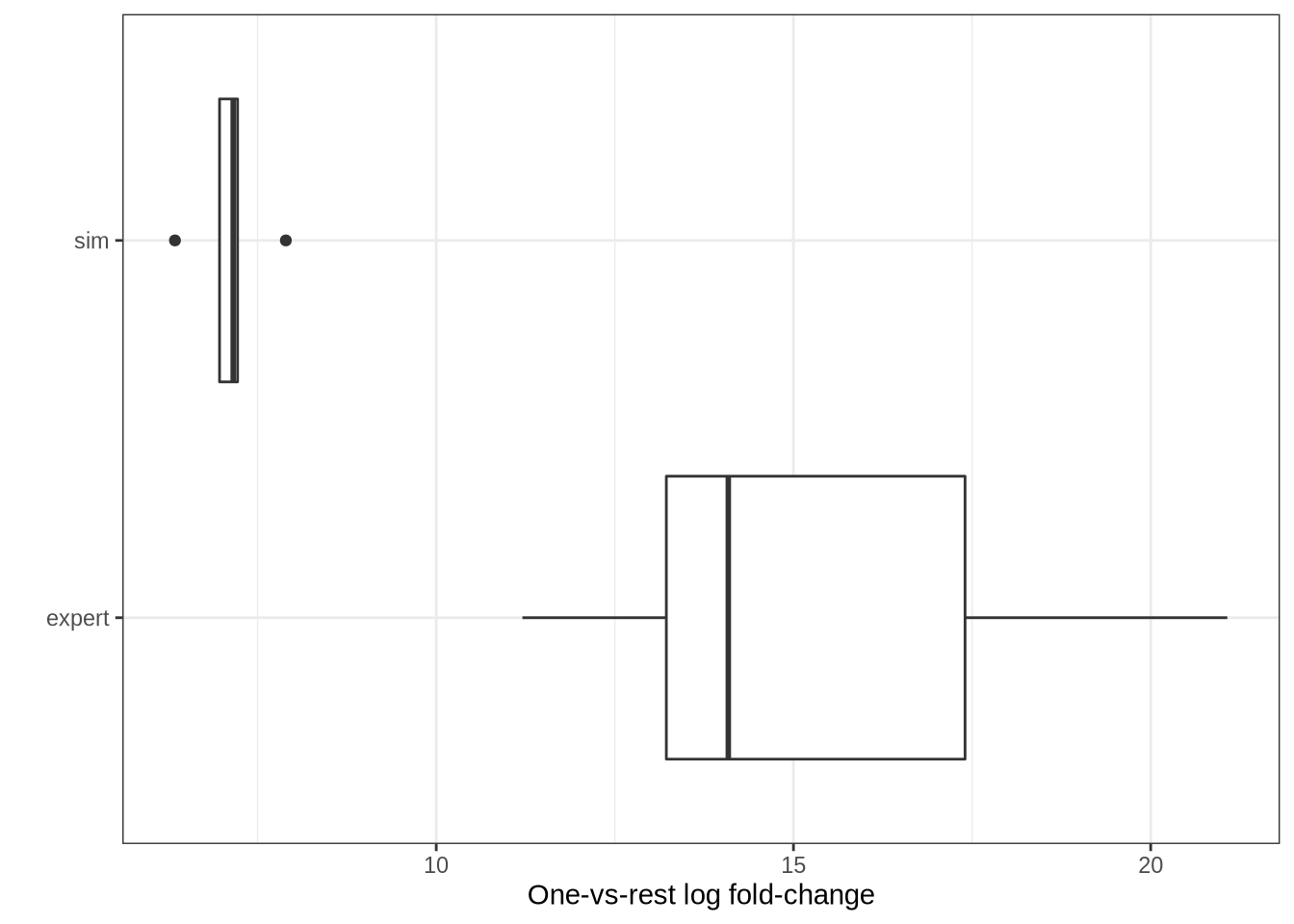
bind_rows(
tibble(type = "sim", logfc = lawlor_top_sim_logfcs),
tibble(type = "expert", logfc = lawlor_top_expert_logfcs)
) %>%
ggplot(aes(x = type, y = logfc)) +
geom_boxplot() +
coord_flip() +
theme_bw() +
labs(
x = "",
y = "One-vs-rest log fold-change"
)
expert_vs_simulated_lfc <- bind_rows(
  tibble(type = "Simulated", data = "Lawlor",
         logfc = lawlor_top_sim_logfcs),
  tibble(type = "Expert-annotated", data = "Lawlor",
         logfc = lawlor_top_expert_logfcs),
  tibble(type = "Simulated", data = "pbmc3k",
         logfc = pbmc3k_top_sim_logfcs),
  tibble(type = "Expert-annotated", data = "pbmc3k",
         logfc = pbmc3k_top_expert_logfcs)
) %>%
  ggplot(aes(x = data, y = logfc, fill = data)) +
  geom_boxplot() +
  coord_flip() +
  facet_grid(rows = vars(type)) +
  theme_bw() +
  labs(
    x = "",
    y = "One-vs-rest log fold-change"
  ) +
  guides(fill = "none")

ggsave(
  here::here("figures", "final", "simulated-vs-expert-lfc.pdf"),
  expert_vs_simulated_lfc,
  width = 12,
  height = 12,
  units = "in"
)
Simulated log fold-change curves
plot_logfc_sim_mgs(pbmc3k_sim, pbmc3k_mg_info) 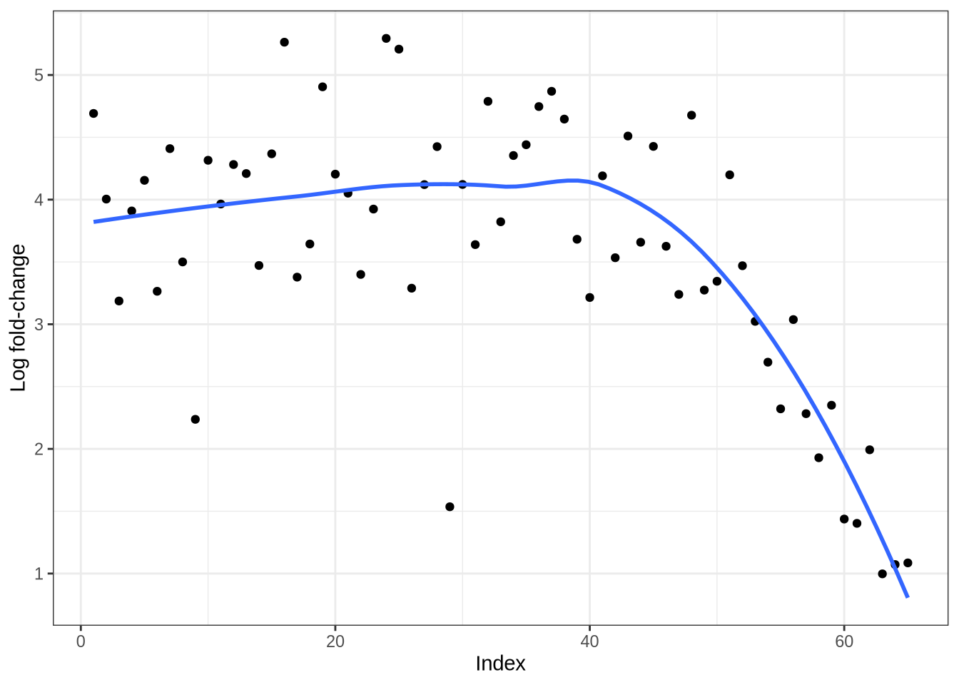
plot_logfc_sim_mgs(zeisel_sim, zeisel_mg_info) 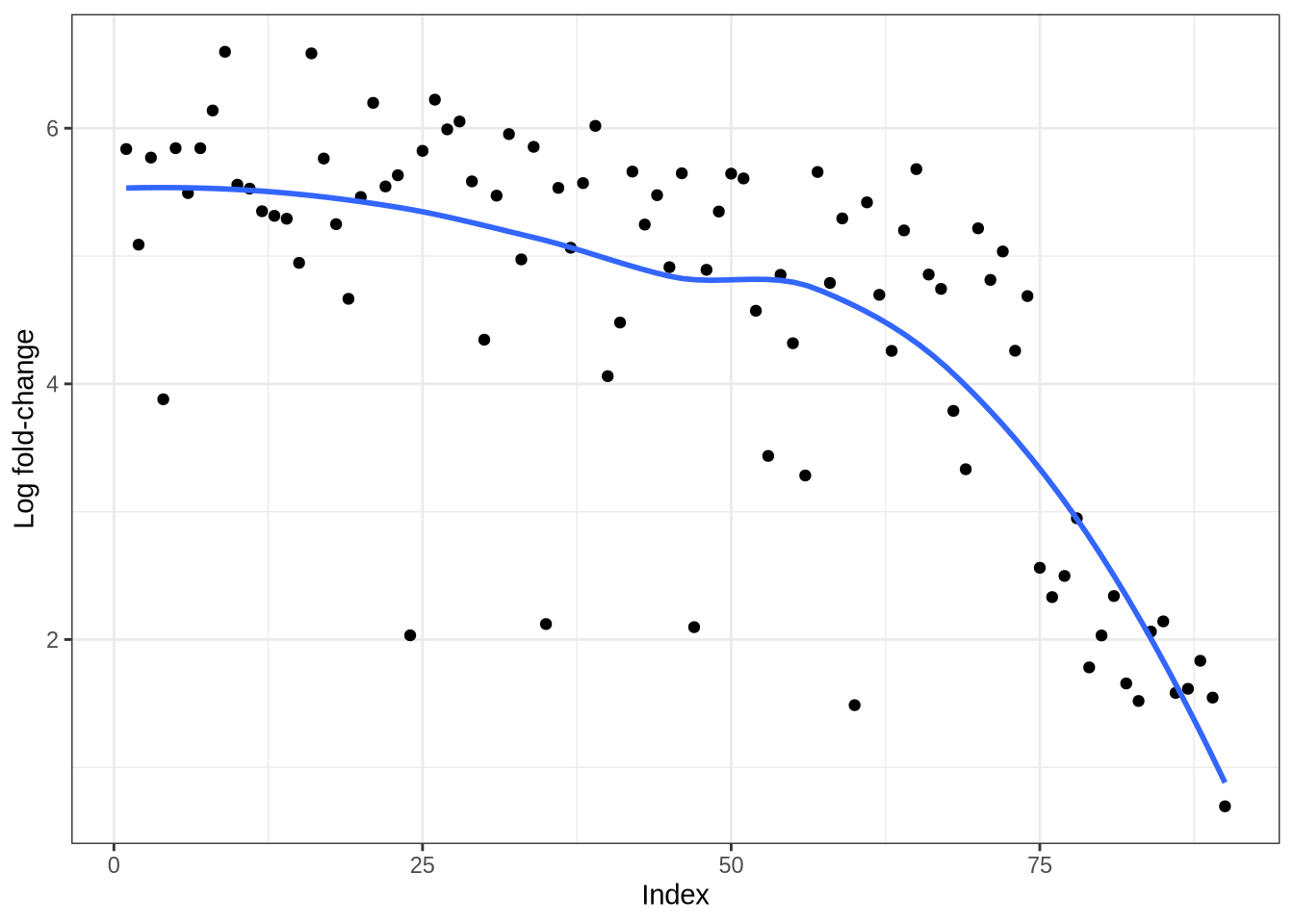
plot_logfc_sim_mgs(lawlor_sim, lawlor_mg_info) 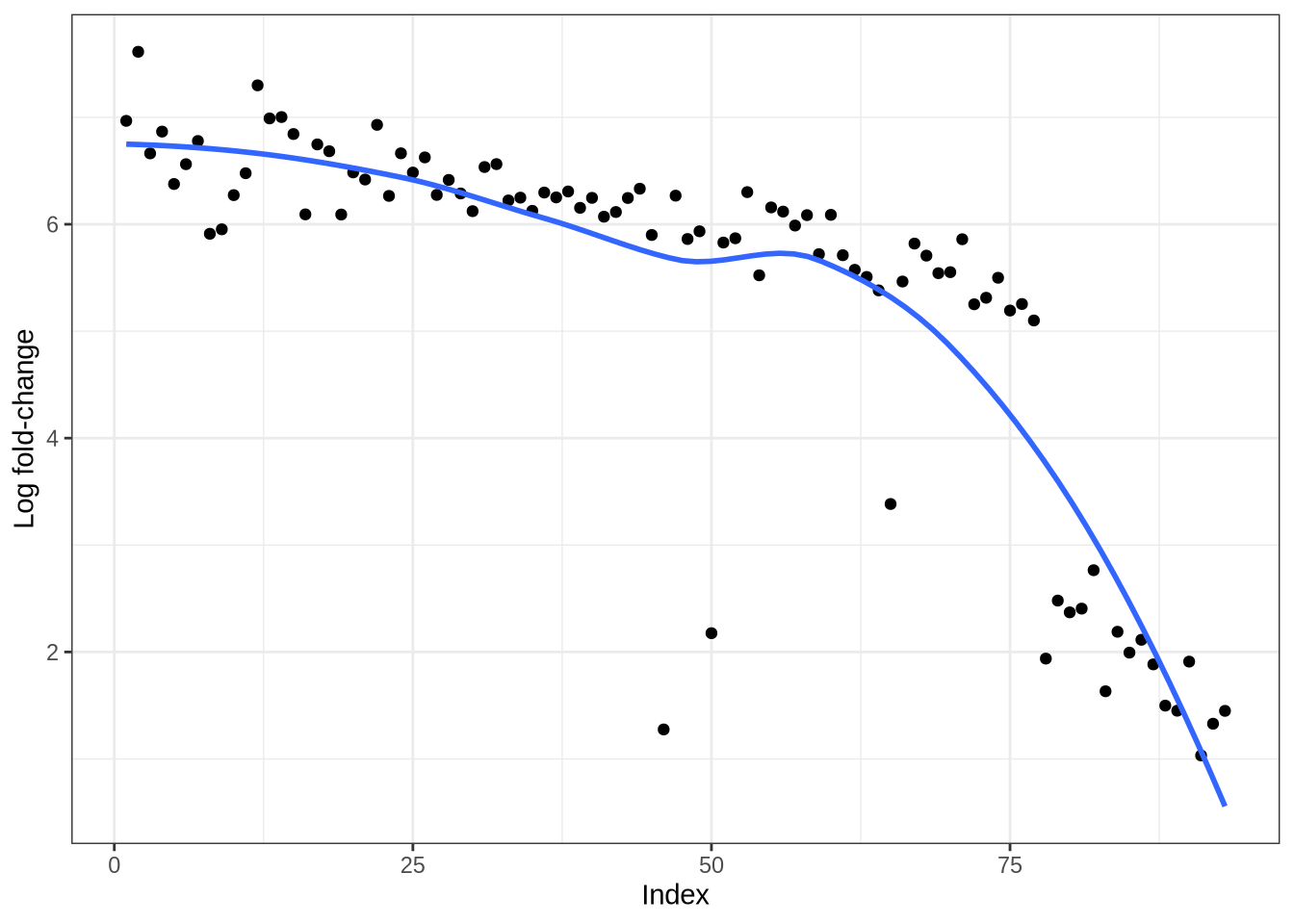
plot_logfc_sim_mgs(endothelial_sim, endothelial_mg_info) 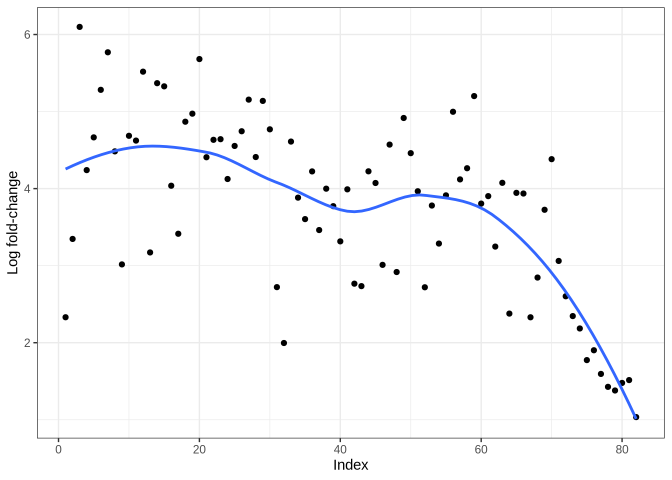
Real log fold-change curves
plot_logfc_real_mgs(pbmc3k, pbmc3k_result, cluster = "B") 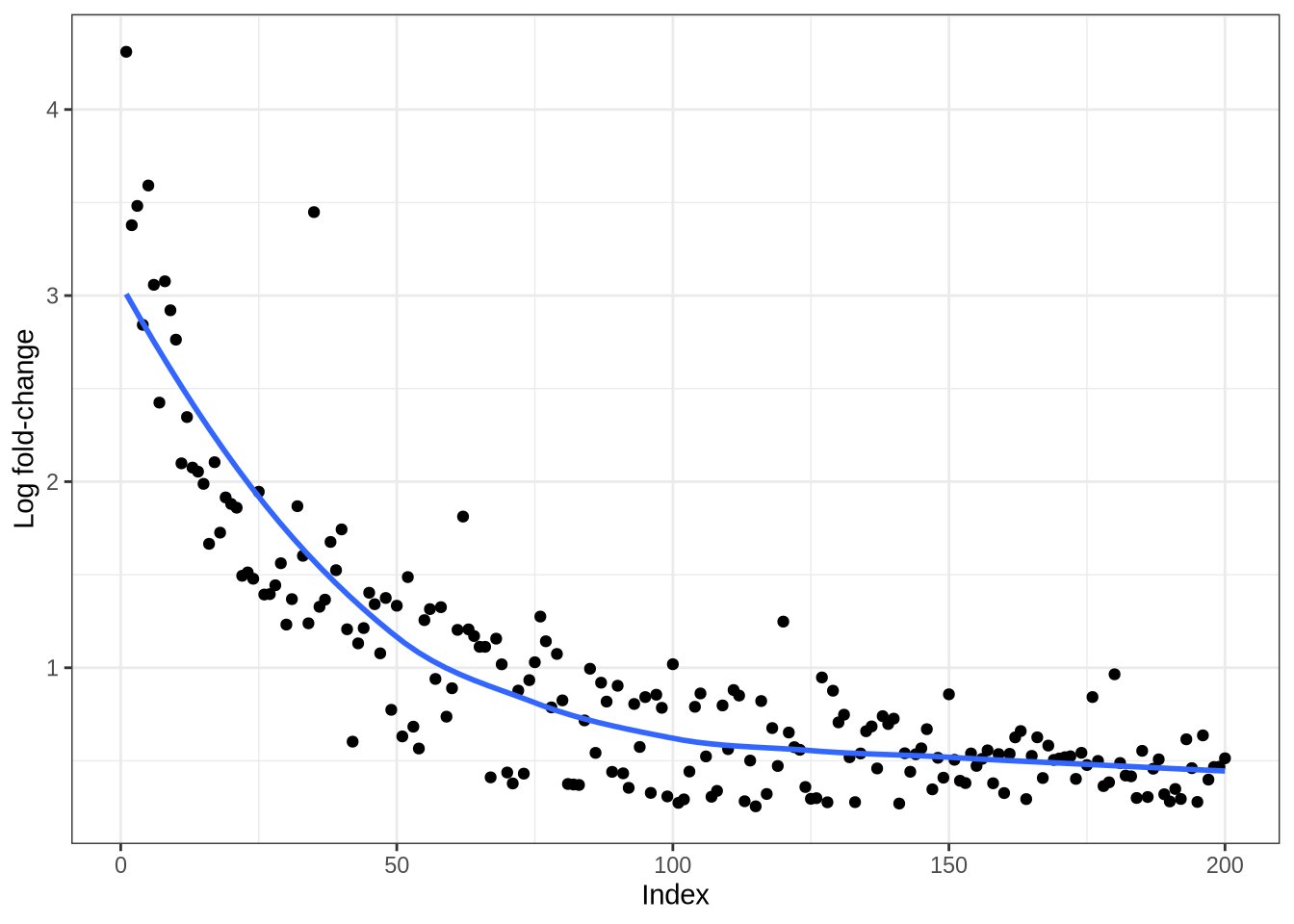
#plot_logfc_real_mgs(zeisel, zeisel_result, cluster = "microglia")
plot_logfc_real_mgs(lawlor, lawlor_result, cluster = "Alpha") 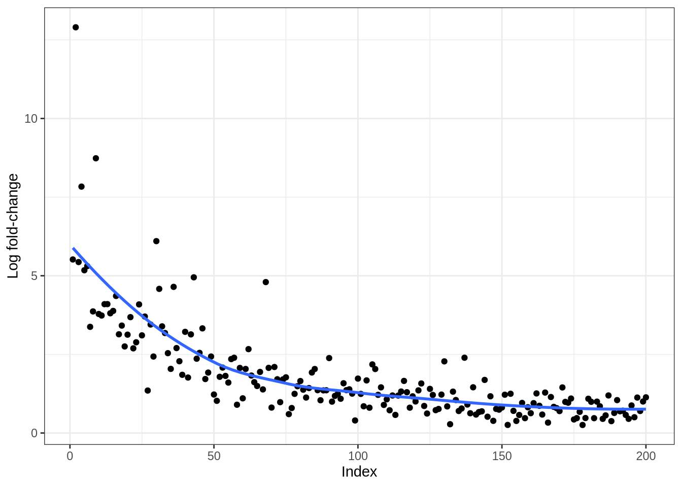
Plot specific cluster examples
plot_specifc_mgs(pbmc3k_sim, pbmc3k_mg_info, c(12, 32, 52))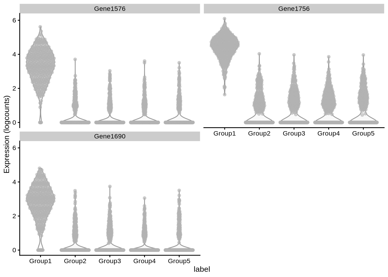
plot_specifc_mgs(zeisel_sim, zeisel_mg_info, c(1, 10, 20))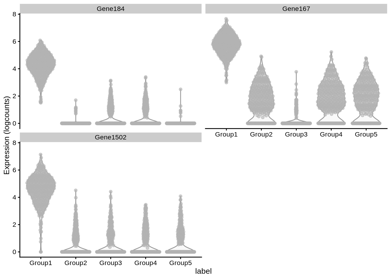
plot_specifc_mgs(lawlor_sim, lawlor_mg_info, c(1, 10, 20))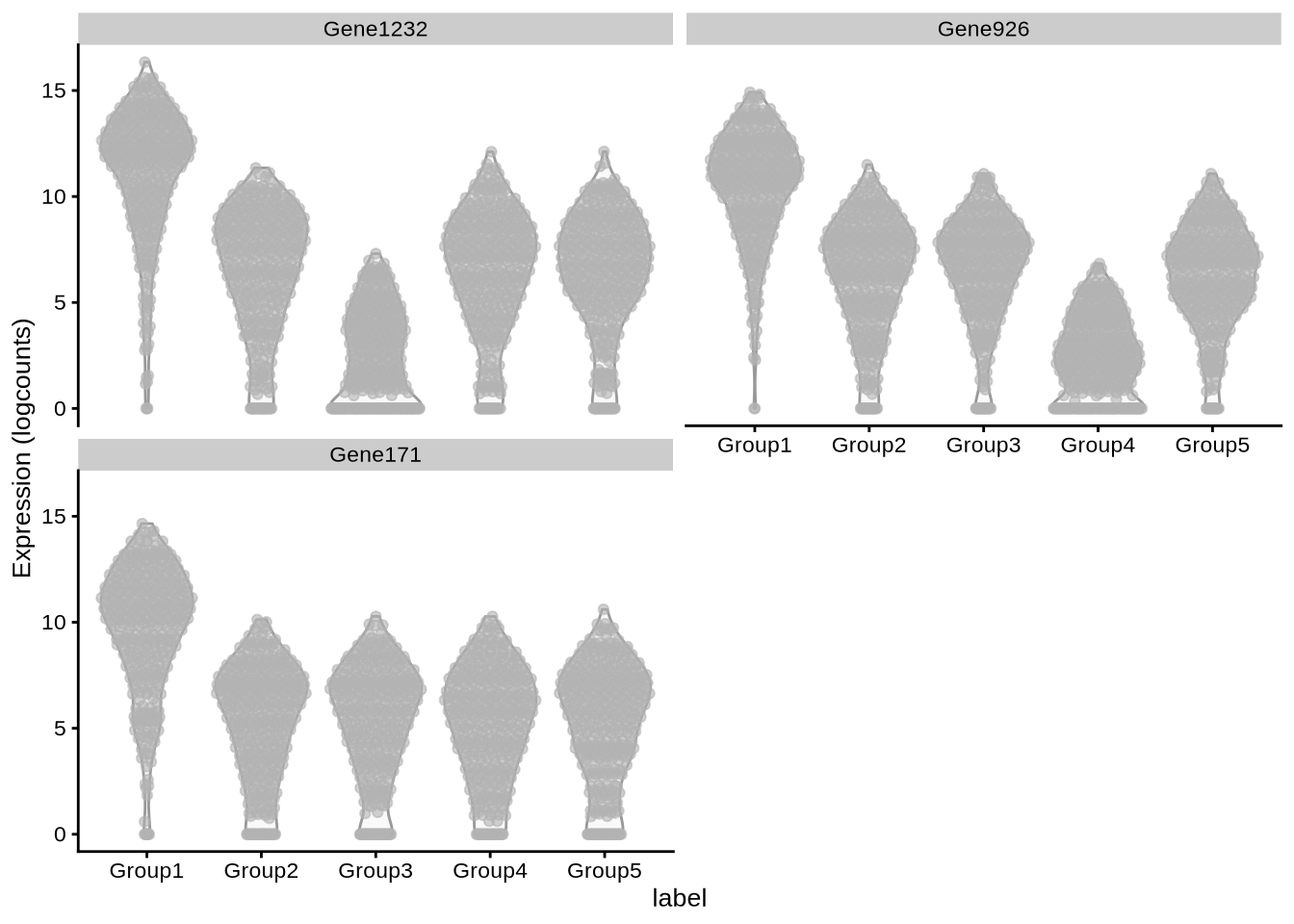
plot_specifc_mgs(lawlor_sim, lawlor_mg_info, c(1, 10, 20))
pbmc3k_mg_info[[1]] %>%
  get_top_true_mgs(n = 20, direction = "up", up_mean_filter = 0.1)
# A tibble: 20 × 8
gene gene_mean fc mean_score median_score max_score direction de_value
<chr> <dbl> <dbl> <dbl> <dbl> <dbl> <chr> <dbl>
1 Gene45 0.313 3.98 3.98 3.17 6.39 up 23.9
2 Gene778 0.216 3.73 3.73 2.91 6.20 up 18.3
3 Gene1916 0.104 3.64 3.64 2.95 5.72 up 19.1
4 Gene82 0.232 3.57 3.57 2.80 5.86 up 16.5
5 Gene1637 0.132 3.48 3.48 3.48 3.48 up 32.5
6 Gene565 0.235 3.47 3.47 2.66 5.88 up 14.3
7 Gene1228 0.175 3.46 3.46 3.46 3.46 up 31.7
8 Gene1087 0.105 3.30 3.30 3.30 3.30 up 27.0
9 Gene189 0.234 3.29 3.29 3.28 6.39 up 26.5
10 Gene37 0.184 3.27 3.27 3.27 3.27 up 26.4
11 Gene823 0.152 3.21 3.21 3.21 3.21 up 24.8
12 Gene1576 0.242 3.20 3.20 3.20 3.20 up 24.5
13 Gene1227 0.200 3.16 3.16 3.16 3.16 up 23.6
14 Gene1904 0.110 3.15 3.15 3.15 3.15 up 23.4
15 Gene1868 0.254 3.15 3.15 3.15 3.15 up 23.3
16 Gene167 0.647 3.14 3.14 3.14 3.14 up 23.1
17 Gene366 0.121 3.13 3.13 3.13 3.13 up 22.9
18 Gene1604 0.145 3.11 3.11 3.11 3.11 up 22.4
19 Gene1481 0.487 3.10 3.10 3.10 3.10 up 22.2
20 Gene1894 0.227 3.09 3.09 3.09 3.09 up 22.0pbmc3k_sim_result$result %>%
filter(cluster == "Group1") %>%
print(n = 30)# A tibble: 510 × 7
p_value p_value_adj cluster log_fc gene raw_statistic scaled_statistic
<dbl> <dbl> <fct> <dbl> <chr> <dbl> <dbl>
1 4.54e-272 9.05e-269 Group1 3.60 Gene1080 0 0
2 3.28e-271 6.54e-268 Group1 3.67 Gene319 0 0
3 9.54e-271 1.90e-267 Group1 3.41 Gene376 0 0
4 1.17e-265 2.33e-262 Group1 3.47 Gene1904 0 0
5 5.14e-265 1.02e-261 Group1 4.15 Gene1637 0 0
6 4.75e-263 9.47e-260 Group1 4.32 Gene37 0 0
7 1.26e-262 2.50e-259 Group1 3.19 Gene1916 0 0
8 9.40e-261 1.87e-257 Group1 3.96 Gene823 0 0
9 1.22e-260 2.42e-257 Group1 4.41 Gene1228 0 0
10 1.40e-260 2.78e-257 Group1 3.64 Gene1604 0 0
11 1.07e-255 2.13e-252 Group1 4.05 Gene158 0 0
12 6.75e-255 1.34e-251 Group1 3.91 Gene82 0 0
13 3.77e-253 7.50e-250 Group1 3.92 Gene467 0 0
14 4.46e-253 8.88e-250 Group1 3.39 Gene1222 0 0
15 2.27e-252 4.52e-249 Group1 4.00 Gene778 0 0
16 2.50e-252 4.98e-249 Group1 4.21 Gene1227 0 0
17 9.19e-252 1.83e-248 Group1 4.69 Gene45 0 0
18 2.36e-250 4.70e-247 Group1 3.05 Gene1050 0 0
19 1.74e-249 3.47e-246 Group1 3.50 Gene1087 0 0
20 2.51e-246 4.99e-243 Group1 4.12 Gene151 0 0
21 3.07e-246 6.12e-243 Group1 3.66 Gene532 0 0
22 8.55e-242 1.70e-238 Group1 4.28 Gene1576 0 0
23 3.57e-241 7.11e-238 Group1 3.40 Gene1250 0 0
24 5.65e-240 1.12e-236 Group1 4.37 Gene1868 0 0
25 7.04e-240 1.40e-236 Group1 2.94 Gene283 0 0
26 1.36e-238 2.70e-235 Group1 4.12 Gene649 0 0
27 4.35e-238 8.67e-235 Group1 3.29 Gene1900 0 0
28 5.47e-238 1.09e-234 Group1 4.43 Gene860 0 0
29 1.38e-236 2.75e-233 Group1 4.20 Gene1894 0 0
30 7.13e-236 1.42e-232 Group1 3.68 Gene841 0 0
# … with 480 more rowspbmc3k_sim_result$result %>%
filter(cluster == "Group1") %>%
mutate(n = 1:n()) %>%
filter(gene %in% c("Gene1270", "Gene46", "Gene865")) %>%
print(n = 30)# A tibble: 1 × 8
p_value p_value_adj cluster log_fc gene raw_statistic scaled_statistic n
<dbl> <dbl> <fct> <dbl> <chr> <dbl> <dbl> <int>
1 3.70e-50 7.38e-47 Group1 -1.50 Gene… 0 0 110plotExpression(pbmc3k_sim, x = "label",
features = c("Gene90", "Gene1413", "Gene1098"))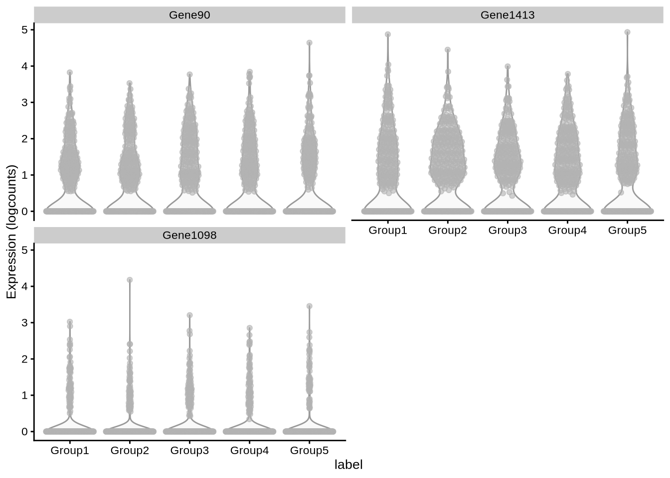
plotExpression(pbmc3k_sim, x = "label",
               features = c("Gene743", "Gene579"))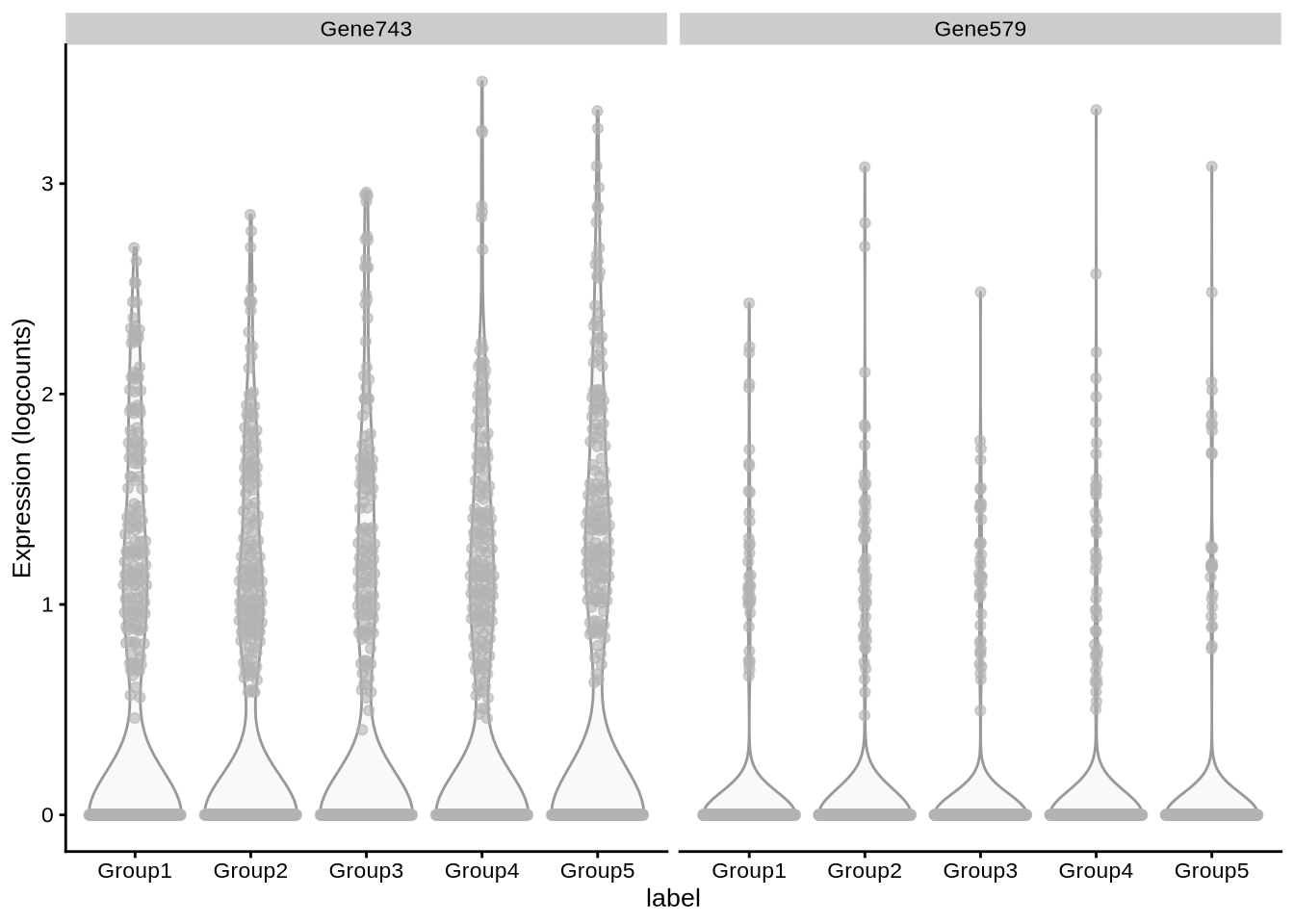
plotExpression(pbmc3k_sim, x = "label",
               features = c("Gene1270", "Gene46", "Gene865"))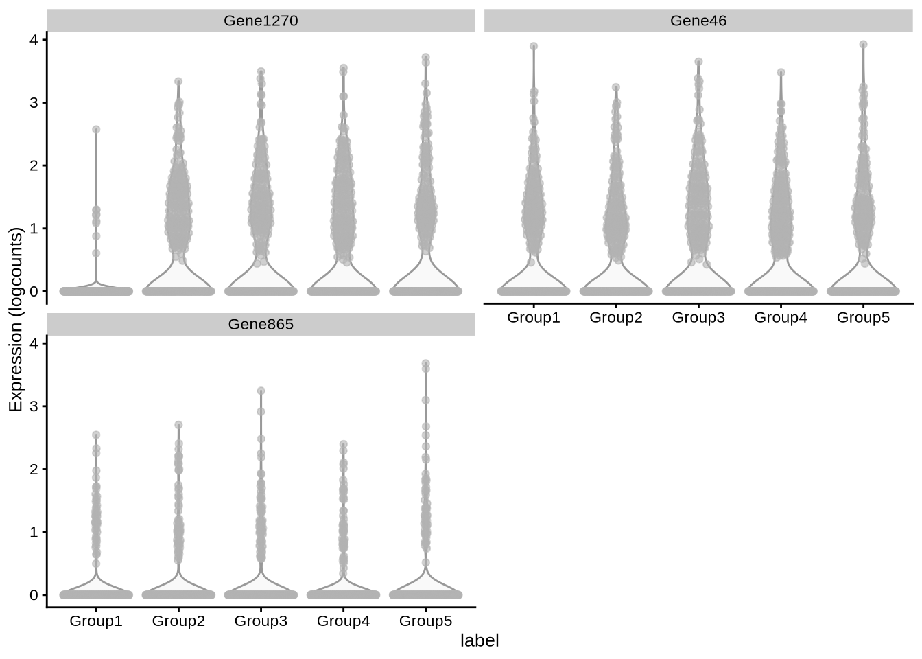
plotExpression(pbmc3k_sim, x = "label",
               features = c("Gene46"))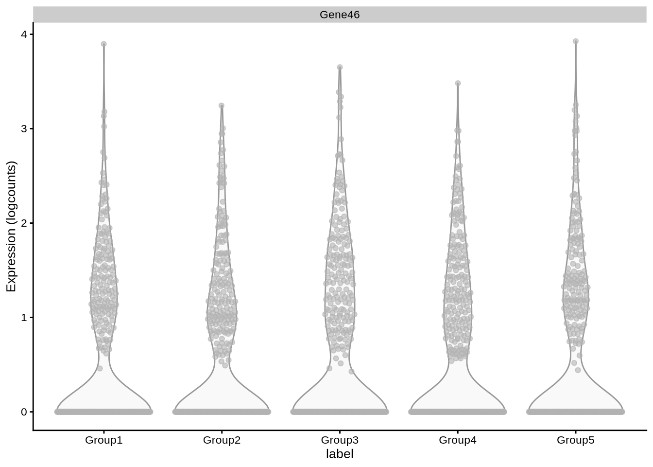
Down-regulated marker genes analysis
lawlor_mg_info %>%
  pluck("group_1") %>%
  filter(gene_mean > 0.1) %>%
  arrange(desc(mean_score))
# A tibble: 2,000 × 8
gene gene_mean fc mean_score median_score max_score direction de_value
<chr> <dbl> <dbl> <dbl> <dbl> <dbl> <chr> <dbl>
1 Gene1232 151. 3.99 3.99 3.24 6.24 up 25.5
2 Gene1840 35.1 3.94 3.94 3.24 6.05 up 25.6
3 Gene65 146. 3.88 3.88 3.05 6.40 up 21.0
4 Gene890 76.8 3.75 3.75 2.95 6.13 up 19.2
5 Gene5 103. 3.71 3.71 2.95 5.98 up 19.1
6 Gene1619 141. 3.70 3.70 2.95 5.97 up 19.1
7 Gene1324 110. 3.64 3.64 2.92 5.80 up 18.5
8 Gene975 117. 3.61 3.61 2.85 5.89 up 17.3
9 Gene786 108. 3.57 3.57 2.88 5.66 up 17.8
10 Gene926 120. 3.55 3.55 2.84 5.69 up 17.1
# … with 1,990 more rowsplotExpression(
lawlor_sim,
x = "label",
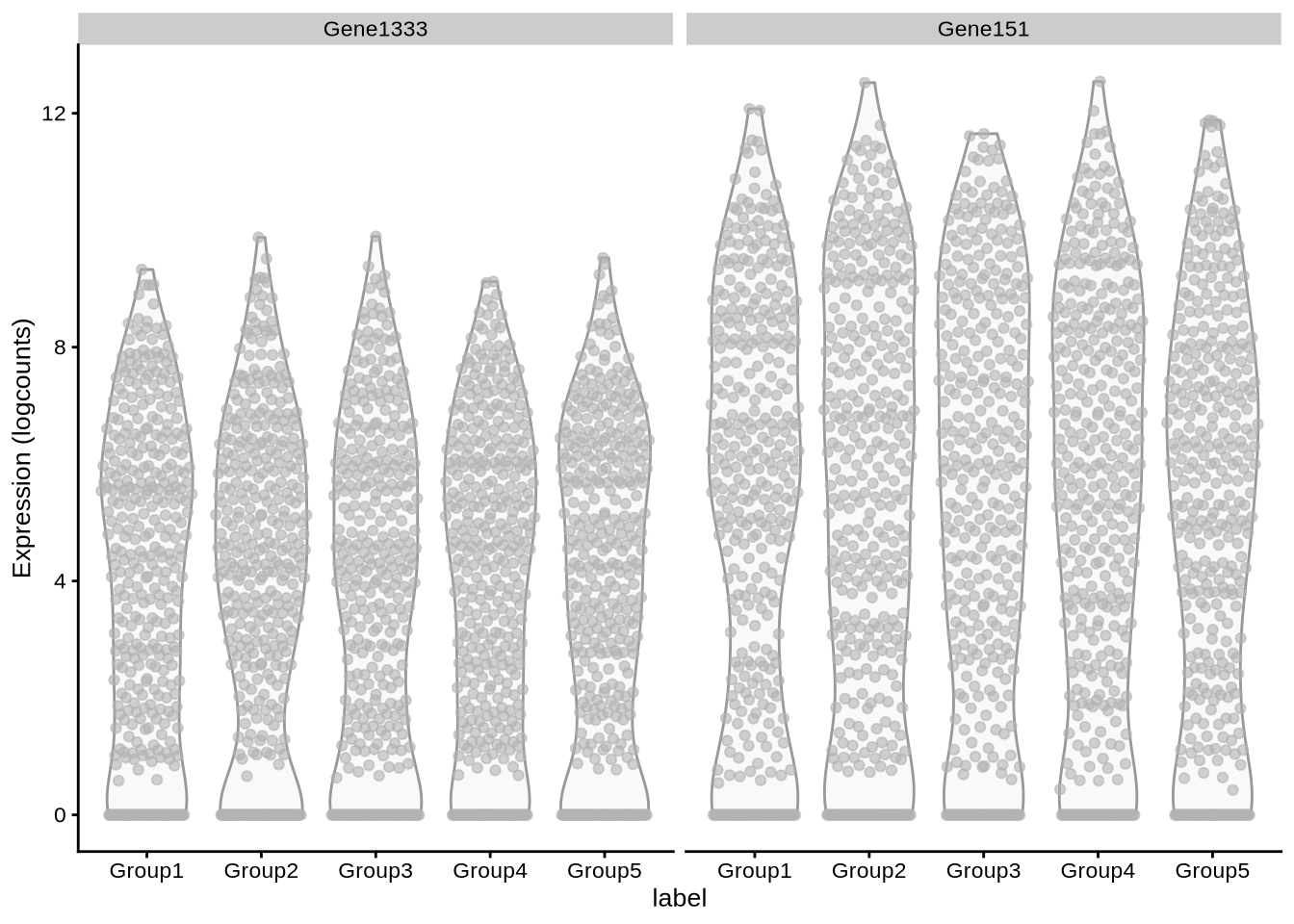
c("Gene1333", "Gene151")
)
zeisel_mg_info %>%
  pluck("group_1") %>%
  filter(gene_mean > 0.1) %>%
  arrange(desc(mean_score))
# A tibble: 1,938 × 8
gene gene_mean fc mean_score median_score max_score direction de_value
<chr> <dbl> <dbl> <dbl> <dbl> <dbl> <chr> <dbl>
1 Gene184 0.523 4.95 4.95 4.87 6.57 up 32.0
2 Gene1031 0.599 4.50 4.50 4.46 6.15 up 19.0
3 Gene1025 0.957 4.03 4.03 3.21 6.49 up 24.8
4 Gene71 0.191 4.00 4.00 3.14 6.57 up 23.1
5 Gene1298 1.18 3.96 3.96 3.18 6.30 up 24.1
6 Gene537 0.818 3.94 3.94 3.19 6.18 up 24.3
7 Gene761 1.98 3.93 3.93 3.05 6.58 up 21.2
8 Gene999 3.49 3.82 3.82 3.10 6.00 up 22.1
9 Gene1203 6.88 3.81 3.81 3.14 5.79 up 23.2
10 Gene167 2.60 3.63 3.63 2.90 5.80 up 18.2
# … with 1,928 more rowsplotExpression(
zeisel_sim,
x = "label",
c("Gene924", "Gene844")
)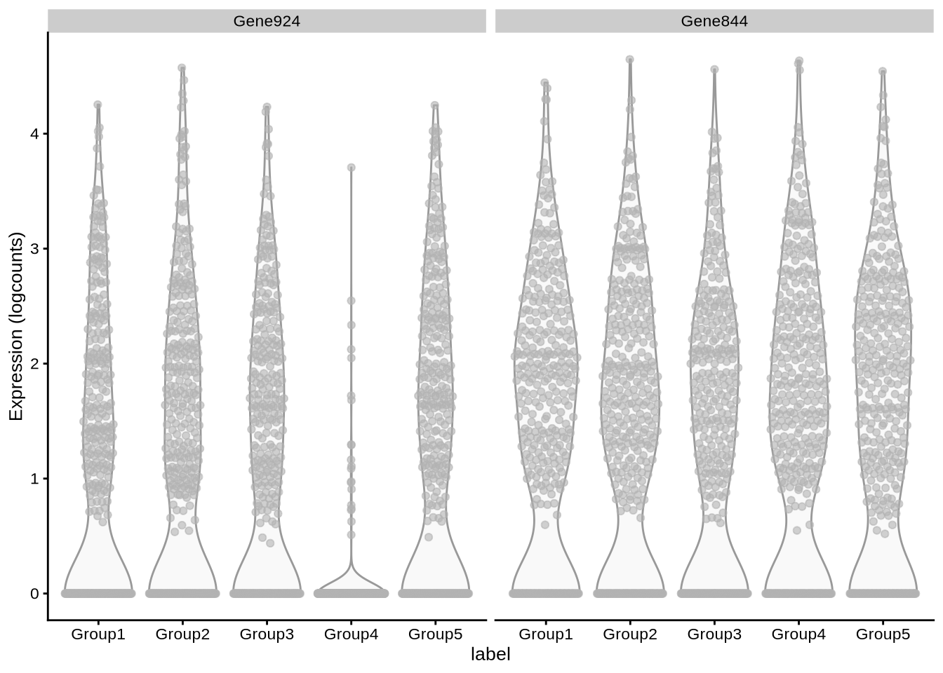
plotExpression(
zeisel_sim,
x = "label",
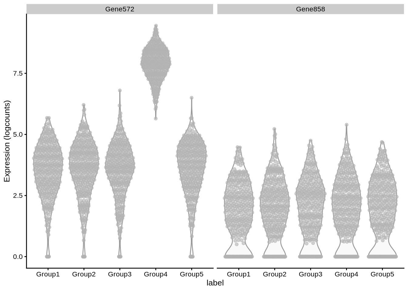
c("Gene572", "Gene858")
)
pbmc3k_mg_info %>%
  pluck("group_1") %>%
  filter(gene_mean > 0.1) %>%
  arrange(mean_score)
# A tibble: 1,275 × 8
gene gene_mean fc mean_score median_score max_score direction de_value
<chr> <dbl> <dbl> <dbl> <dbl> <dbl> <chr> <dbl>
1 Gene1638 0.391 -4.13 -4.13 -3.33 -3.33 down 0.0358
2 Gene1011 0.381 -3.91 -3.91 -3.18 -3.18 down 0.0418
3 Gene626 0.126 -3.83 -3.83 -3.05 -3.05 down 0.0473
4 Gene1251 0.155 -3.78 -3.78 -2.96 -2.96 down 0.0516
5 Gene141 0.104 -3.71 -3.71 -2.92 -2.92 down 0.0539
6 Gene548 0.391 -3.60 -3.60 -2.90 -2.90 down 0.0551
7 Gene342 0.206 -3.54 -3.54 -2.79 -2.79 down 0.0615
8 Gene1623 0.936 -3.48 -3.48 -2.66 -2.66 down 0.0696
9 Gene60 0.589 -3.47 -3.47 -3.47 -3.47 down 0.0312
10 Gene1435 0.642 -3.46 -3.46 -3.46 -3.46 down 0.0313
# … with 1,265 more rowsplotExpression(
pbmc3k_sim,
x = "label",
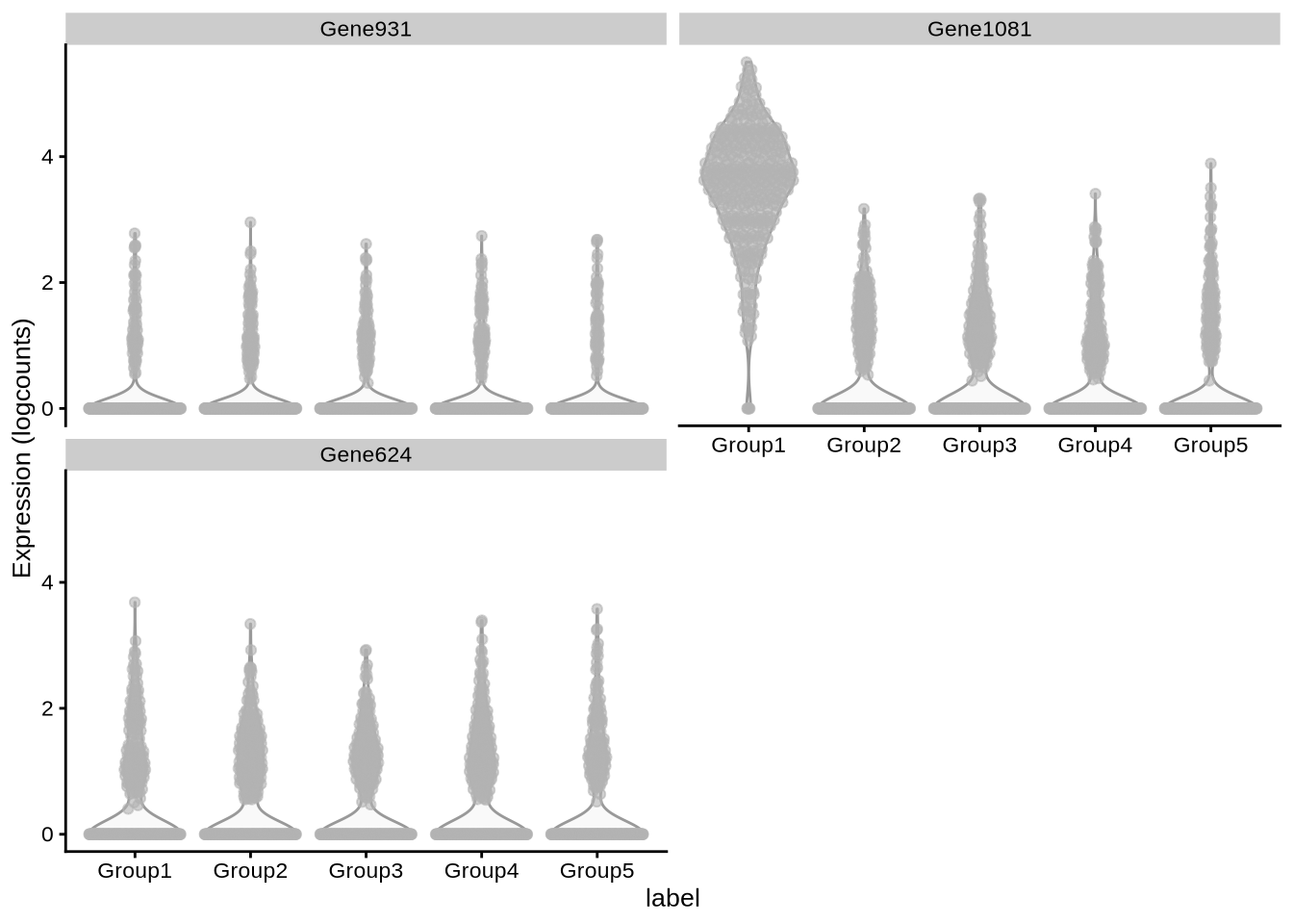
c("Gene931", "Gene1081", "Gene624")
)
Gene mean filtering analysis
pbmc3k_sim$Group <- substr(
  pbmc3k_sim$label,
  6,
  6
)

mgs_no_mean_filter <- pbmc3k_mg_info %>%
  pluck("group_1") %>%
  arrange(desc(mean_score)) %>%
  dplyr::slice(1:4) %>%
  pull(gene)

mgs_with_mean_filter <- pbmc3k_mg_info %>%
  pluck("group_1") %>%
  filter(gene_mean > 0.05) %>%
  arrange(desc(mean_score)) %>%
  dplyr::slice(1:4) %>%
  pull(gene)

no_mean_filter_plot <- plotExpression(
  pbmc3k_sim,
  x = "Group",
  mgs_no_mean_filter
) +
  labs(
    title = "Without mean filter"
  )

with_mean_filter_plot <- plotExpression(
  pbmc3k_sim,
  x = "Group",
  mgs_with_mean_filter
) +
  labs(
    title = "With mean filter"
  )

no_mean_filter_plot + with_mean_filter_plot +
  plot_annotation(tag_levels = "a") &
  theme(plot.tag = element_text(size = 18))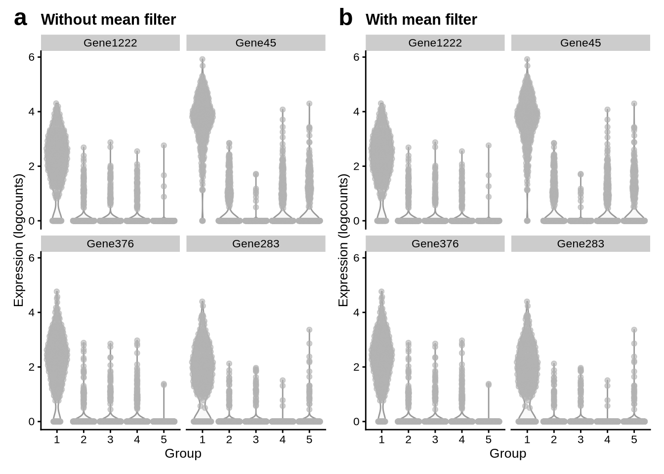
# standard_sim_1_pbmc3k_seurat_wilcox <- readRDS(
#   here::here("results", "sim_data",
#              "standard_sim_1-pbmc3k-seurat_wilcox.rds")
# )
#
# standard_sim_1_pbmc3k_seurat_t <- readRDS(
#   here::here("results", "sim_data",
#              "standard_sim_1-pbmc3k-seurat_t.rds")
# )
#
# n <- 40
#
# seurat_wilcox_log_fc <- standard_sim_1_pbmc3k_seurat_wilcox %>%
#   pluck("result") %>%
#   filter(cluster == "Group1") %>%
#   filter(log_fc > 0) %>%
#   dplyr::slice(1:n) %>%
#   pull(log_fc)
#
# seurat_t_log_fc <- standard_sim_1_pbmc3k_seurat_t %>%
#   pluck("result") %>%
#   filter(cluster == "Group1") %>%
#   filter(log_fc > 0) %>%
#   dplyr::slice(1:n) %>%
#   pull(log_fc)
#
# top_mgs_seurat_wilcox <- standard_sim_1_pbmc3k_seurat_wilcox %>%
#   pluck("result") %>%
#   filter(cluster == "Group1") %>%
#   filter(log_fc > 0) %>%
#   dplyr::slice(1:n) %>%
#   pull(gene)
#
# top_mgs_no_filter <- mg_info_standard_sim_1_pbmc3k %>%
#   pluck("group_1") %>%
#   arrange(desc(mean_score)) %>%
#   dplyr::slice(1:n) %>%
#   pull(gene)
#
# top_mgs_no_filter_log_fc <- standard_sim_1_pbmc3k_seurat_wilcox %>%
#   pluck("result") %>%
#   filter(cluster == "Group1") %>%
#   filter(gene %in% top_mgs_no_filter) %>%
#   pull(log_fc)
#
#
# top_mgs_no_filter_log_fc[[40]] <- mean(top_mgs_no_filter_log_fc)
#
# top_mgs_with_filter <- mg_info_standard_sim_1_pbmc3k %>%
#   pluck("group_1") %>%
#   filter(gene_mean > 0.1) %>%
#   arrange(desc(mean_score)) %>%
#   dplyr::slice(1:n) %>%
#   pull(gene)
#
# top_mgs_with_filter_log_fc <- standard_sim_1_pbmc3k_seurat_wilcox %>%
#   pluck("result") %>%
#   filter(cluster == "Group1") %>%
#   filter(gene %in% top_mgs_with_filter) %>%
#   pull(log_fc)
#
# tibble(
#   filter_logfc = top_mgs_with_filter_log_fc,
#   nofilter_logfc = top_mgs_no_filter_log_fc,
#   wilcox_logfc = seurat_wilcox_log_fc,
#   t_logfc = seurat_t_log_fc,
# ) %>%
#   pivot_longer(
#     cols = everything(),
#     names_pattern = "(.*)_.*",
#     values_to = "log_fc",
#     names_to = "method"
#   ) %>%
#   mutate(score = if_else(
#     method %in% c("filter", "nofilter"),
#     "Scored",
#     "Selected"
#     )
#   ) %>%
#   mutate(method = case_when(
#     method == "filter" ~ "With mean filter",
#     method == "nofilter" ~ "Without mean filter",
#     method == "t" ~ "Seurat t-test",
#     method == "wilcox" ~ "Seurat Wilcoxon"
#   )) %>%
#   ggplot(aes(x = factor(method), y = log_fc, fill = score)) +
#   geom_boxplot() +
#   coord_flip() +
#   labs(
#     fill = "Method",
#     y = "One-vs-rest log fold change",
#     x = "Marker gene type"
#   ) +
#   scale_y_continuous(breaks = c(1, 2, 4, 6)) +
#   theme_bw()
# top_mgs_with_filter <- mg_info_standard_sim_1_pbmc3k %>%
# pluck("group_1") %>%
# filter(gene_mean > 0.1) %>%
# arrange(desc(mean_score)) %>%
# dplyr::slice(1:80) %>%
# mutate(rank = 1:n())
#
# m_1 <- rowMeans(
# expm1(logcounts(sim_1_pbmc3k[, sim_1_pbmc3k$label == "Group1"]))
# )
# m_2 <- rowMeans(
# expm1(logcounts(sim_1_pbmc3k[, sim_1_pbmc3k$label != "Group1"]))
# )
# log_fcs <- log(m_1 + 1, base = 2) - log(m_2 + 1, base = 2)
# log_fcs_tib <- tibble(gene = rownames(sim_1_pbmc3k), log_fc = log_fcs)
#
# top_mgs_with_filter <- top_mgs_with_filter %>%
# left_join(log_fcs_tib, by = "gene")
#
# top_mgs_with_filter %>%
# ggplot(aes(x = rank, y = log_fc)) +
# geom_point(colour = "seagreen") +
# geom_smooth(method = "loess", formula = y ~ x) +
# labs(
# x = "True marker gene rank",
# y = "Two sample log fold change"
# ) +
# theme_bw()
# ```
#
#
# ```{r mean-histogram}
# mg_info_standard_sim_1_pbmc3k %>%
# pluck("group_1") %>%
# ggplot(aes(x = gene_mean)) +
# geom_histogram(
# bins = 20,
# fill = "seagreen",
# colour = "black"
# ) +
# labs(
# x = "Gene mean",
# y = "Count",
# title = "Histogram of simulated gene means"
# ) +
# theme_bw()
#
# standard_sim_1_pbmc3k %>%
# logcounts() %>%
# rowMeans() %>%
# tibble() %>%
# setNames("mean") %>%
# ggplot(aes(x = mean)) +
# geom_histogram()
devtools::session_info()─ Session info ──────────────────────────────────────────────────────────────
hash: tear-off calendar, railway car, person in bed: dark skin tone
setting value
version R version 4.1.2 (2021-11-01)
os Red Hat Enterprise Linux 9.2 (Plow)
system x86_64, linux-gnu
ui X11
language (EN)
collate en_AU.UTF-8
ctype en_AU.UTF-8
tz Australia/Melbourne
date 2024-01-01
pandoc 2.18 @ /apps/easybuild-2022/easybuild/software/MPI/GCC/11.3.0/OpenMPI/4.1.4/RStudio-Server/2022.07.2+576-Java-11-R-4.1.2/bin/pandoc/ (via rmarkdown)
─ Packages ───────────────────────────────────────────────────────────────────
package * version date (UTC) lib source
assertthat 0.2.1 2019-03-21 [2] CRAN (R 4.1.2)
beachmat 2.10.0 2021-10-26 [1] Bioconductor
beeswarm 0.4.0 2021-06-01 [2] CRAN (R 4.1.2)
Biobase * 2.54.0 2021-10-26 [1] Bioconductor
BiocGenerics * 0.40.0 2021-10-26 [1] Bioconductor
BiocNeighbors 1.12.0 2021-10-26 [1] Bioconductor
BiocParallel 1.28.3 2021-12-09 [1] Bioconductor
BiocSingular 1.10.0 2021-10-26 [1] Bioconductor
bitops 1.0-7 2021-04-24 [2] CRAN (R 4.1.2)
bslib 0.3.1 2021-10-06 [1] CRAN (R 4.1.0)
cachem 1.0.6 2021-08-19 [1] CRAN (R 4.1.0)
callr 3.7.0 2021-04-20 [2] CRAN (R 4.1.2)
cli 3.6.1 2023-03-23 [1] CRAN (R 4.1.0)
colorspace 2.1-0 2023-01-23 [1] CRAN (R 4.1.0)
cowplot 1.1.1 2020-12-30 [2] CRAN (R 4.1.2)
crayon 1.5.1 2022-03-26 [1] CRAN (R 4.1.0)
DBI 1.1.2 2021-12-20 [1] CRAN (R 4.1.0)
DelayedArray 0.20.0 2021-10-26 [1] Bioconductor
DelayedMatrixStats 1.16.0 2021-10-26 [1] Bioconductor
desc 1.4.0 2021-09-28 [2] CRAN (R 4.1.2)
devtools 2.4.2 2021-06-07 [2] CRAN (R 4.1.2)
digest 0.6.29 2021-12-01 [1] CRAN (R 4.1.0)
dplyr * 1.0.9 2022-04-28 [1] CRAN (R 4.1.0)
ellipsis 0.3.2 2021-04-29 [2] CRAN (R 4.1.2)
evaluate 0.14 2019-05-28 [2] CRAN (R 4.1.2)
fansi 1.0.4 2023-01-22 [1] CRAN (R 4.1.0)
farver 2.1.1 2022-07-06 [1] CRAN (R 4.1.0)
fastmap 1.1.0 2021-01-25 [2] CRAN (R 4.1.2)
fs 1.5.2 2021-12-08 [1] CRAN (R 4.1.0)
generics 0.1.3 2022-07-05 [1] CRAN (R 4.1.0)
GenomeInfoDb * 1.30.0 2021-10-26 [1] Bioconductor
GenomeInfoDbData 1.2.7 2021-12-03 [1] Bioconductor
GenomicRanges * 1.46.1 2021-11-18 [1] Bioconductor
ggbeeswarm 0.6.0 2017-08-07 [2] CRAN (R 4.1.2)
ggplot2 * 3.3.6 2022-05-03 [1] CRAN (R 4.1.0)
ggrepel 0.9.1 2021-01-15 [2] CRAN (R 4.1.2)
git2r 0.28.0 2021-01-10 [2] CRAN (R 4.1.2)
glue 1.6.0 2021-12-17 [1] CRAN (R 4.1.0)
gridExtra 2.3 2017-09-09 [2] CRAN (R 4.1.2)
gtable 0.3.0 2019-03-25 [2] CRAN (R 4.1.2)
here 1.0.1 2020-12-13 [1] CRAN (R 4.1.0)
highr 0.9 2021-04-16 [2] CRAN (R 4.1.2)
htmltools 0.5.2 2021-08-25 [1] CRAN (R 4.1.0)
httpuv 1.6.5 2022-01-05 [1] CRAN (R 4.1.0)
IRanges * 2.28.0 2021-10-26 [1] Bioconductor
irlba 2.3.5 2021-12-06 [1] CRAN (R 4.1.0)
jquerylib 0.1.4 2021-04-26 [2] CRAN (R 4.1.2)
jsonlite 1.8.0 2022-02-22 [1] CRAN (R 4.1.0)
knitr 1.36 2021-09-29 [1] CRAN (R 4.1.0)
labeling 0.4.2 2020-10-20 [2] CRAN (R 4.1.2)
later 1.3.0 2021-08-18 [1] CRAN (R 4.1.0)
lattice 0.20-45 2021-09-22 [2] CRAN (R 4.1.2)
lifecycle 1.0.1 2021-09-24 [1] CRAN (R 4.1.0)
magrittr 2.0.3 2022-03-30 [1] CRAN (R 4.1.0)
Matrix 1.3-4 2021-06-01 [2] CRAN (R 4.1.2)
MatrixGenerics * 1.6.0 2021-10-26 [1] Bioconductor
matrixStats * 0.62.0 2022-04-19 [1] CRAN (R 4.1.0)
memoise 2.0.1 2021-11-26 [1] CRAN (R 4.1.0)
mgcv 1.8-38 2021-10-06 [2] CRAN (R 4.1.2)
munsell 0.5.0 2018-06-12 [2] CRAN (R 4.1.2)
nlme 3.1-153 2021-09-07 [2] CRAN (R 4.1.2)
patchwork * 1.1.1 2020-12-17 [2] CRAN (R 4.1.2)
pillar 1.7.0 2022-02-01 [1] CRAN (R 4.1.0)
pkgbuild 1.2.0 2020-12-15 [2] CRAN (R 4.1.2)
pkgconfig 2.0.3 2019-09-22 [2] CRAN (R 4.1.2)
pkgload 1.2.3 2021-10-13 [2] CRAN (R 4.1.2)
prettyunits 1.1.1 2020-01-24 [2] CRAN (R 4.1.2)
processx 3.5.2 2021-04-30 [2] CRAN (R 4.1.2)
promises 1.2.0.1 2021-02-11 [2] CRAN (R 4.1.2)
ps 1.7.1 2022-06-18 [1] CRAN (R 4.1.0)
purrr * 0.3.4 2020-04-17 [2] CRAN (R 4.1.2)
R6 2.5.1 2021-08-19 [1] CRAN (R 4.1.0)
Rcpp 1.0.8.3 2022-03-17 [1] CRAN (R 4.1.0)
RCurl 1.98-1.5 2021-09-17 [1] CRAN (R 4.1.0)
remotes 2.4.2 2021-11-30 [1] CRAN (R 4.1.0)
rlang 1.0.3 2022-06-27 [1] CRAN (R 4.1.0)
rmarkdown 2.14 2022-04-25 [1] CRAN (R 4.1.0)
rprojroot 2.0.3 2022-04-02 [1] CRAN (R 4.1.0)
rstudioapi 0.14 2022-08-22 [1] CRAN (R 4.1.0)
rsvd 1.0.5 2021-04-16 [1] CRAN (R 4.1.0)
S4Vectors * 0.32.3 2021-11-21 [1] Bioconductor
sass 0.4.1 2022-03-23 [1] CRAN (R 4.1.0)
ScaledMatrix 1.2.0 2021-10-26 [1] Bioconductor
scales 1.2.1 2022-08-20 [1] CRAN (R 4.1.0)
scater * 1.22.0 2021-10-26 [1] Bioconductor
scuttle * 1.4.0 2021-10-26 [1] Bioconductor
sessioninfo 1.2.0 2021-10-31 [2] CRAN (R 4.1.2)
SingleCellExperiment * 1.16.0 2021-10-26 [1] Bioconductor
sparseMatrixStats 1.6.0 2021-10-26 [1] Bioconductor
stringi 1.7.6 2021-11-29 [1] CRAN (R 4.1.0)
stringr 1.4.0 2019-02-10 [2] CRAN (R 4.1.2)
SummarizedExperiment * 1.24.0 2021-10-26 [1] Bioconductor
testthat 3.1.0 2021-10-04 [2] CRAN (R 4.1.2)
tibble 3.1.7 2022-05-03 [1] CRAN (R 4.1.0)
tidyr * 1.2.0 2022-02-01 [1] CRAN (R 4.1.0)
tidyselect 1.1.2 2022-02-21 [1] CRAN (R 4.1.0)
usethis 2.1.3 2021-10-27 [2] CRAN (R 4.1.2)
utf8 1.2.3 2023-01-31 [1] CRAN (R 4.1.0)
vctrs 0.4.1 2022-04-13 [1] CRAN (R 4.1.0)
vipor 0.4.5 2017-03-22 [2] CRAN (R 4.1.2)
viridis 0.6.2 2021-10-13 [1] CRAN (R 4.1.0)
viridisLite 0.4.2 2023-05-02 [1] CRAN (R 4.1.0)
whisker 0.4 2019-08-28 [2] CRAN (R 4.1.2)
withr 2.5.0 2022-03-03 [1] CRAN (R 4.1.0)
workflowr 1.7.0 2021-12-21 [1] CRAN (R 4.1.0)
xfun 0.31 2022-05-10 [1] CRAN (R 4.1.0)
XVector 0.34.0 2021-10-26 [1] Bioconductor
yaml 2.3.5 2022-02-21 [1] CRAN (R 4.1.0)
zlibbioc 1.40.0 2021-10-26 [1] Bioconductor
[1] /home/jpullin/R/x86_64-pc-linux-gnu-library/4.1
[2] /apps/easybuild-2022/easybuild/software/MPI/GCC/11.3.0/OpenMPI/4.1.4/R/4.1.2/lib64/R/library
──────────────────────────────────────────────────────────────────────────────