SVI-SAHMRI scRNA-seq analysis workshop

workflowr

• Summary
• Checks
• Past versions

Last updated: 2021-07-07

Checks: 7 0

Knit directory: svi-sahmri_scrna-seq-workshop_2021-july/

This reproducible R Markdown analysis was created with workflowr (version 1.6.2). The Checks tab describes the reproducibility checks that were applied when the results were created. The Past versions tab lists the development history.

---

R Markdown file: up-to-date

Great! Since the R Markdown file has been committed to the Git repository, you know the exact version of the code that produced these results.

Environment: empty

Great job! The global environment was empty. Objects defined in the global environment can affect the analysis in your R Markdown file in unknown ways. For reproduciblity it’s best to always run the code in an empty environment.

Seed: set.seed(20190102)

The command set.seed(20190102) was run prior to running the code in the R Markdown file. Setting a seed ensures that any results that rely on randomness, e.g. subsampling or permutations, are reproducible.

Session information: recorded

Great job! Recording the operating system, R version, and package versions is critical for reproducibility.

Cache: none

Nice! There were no cached chunks for this analysis, so you can be confident that you successfully produced the results during this run.

File paths: relative

Great job! Using relative paths to the files within your workflowr project makes it easier to run your code on other machines.

Repository version: d13d36f

Great! You are using Git for version control. Tracking code development and connecting the code version to the results is critical for reproducibility.

The results in this page were generated with repository version d13d36f. See the Past versions tab to see a history of the changes made to the R Markdown and HTML files.

Note that you need to be careful to ensure that all relevant files for the analysis have been committed to Git prior to generating the results (you can use wflow_publish or wflow_git_commit). workflowr only checks the R Markdown file, but you know if there are other scripts or data files that it depends on. Below is the status of the Git repository when the results were generated:

Ignored files:
    Ignored:    .Rhistory
    Ignored:    .Rproj.user/

Untracked files:
    Untracked:  raw_data/
    Untracked:  svi-sahmri_scrna-seq-workshop_2021-july.Rproj
    Untracked:  untar_path/

Unstaged changes:
    Modified:   analysis/_site.yml

Note that any generated files, e.g. HTML, png, CSS, etc., are not included in this status report because it is ok for generated content to have uncommitted changes.

---

These are the previous versions of the repository in which changes were made to the R Markdown (analysis/sahmri_analysis-workflow.Rmd) and HTML (public/sahmri_analysis-workflow.html) files. If you’ve configured a remote Git repository (see ?wflow_git_remote), click on the hyperlinks in the table below to view the files as they were in that past version.

File	Version	Author	Date	Message
Rmd	d13d36f	Davis McCarthy	2021-07-07	Updating workshop content
html	9ec2636	Davis McCarthy	2021-07-05	Substantial updates to workflow
Rmd	03e7bf9	Davis McCarthy	2021-07-05	Major update of normalisation section and more tidying
html	752aaa3	Davis McCarthy	2021-07-05	Updating workflowr website
Rmd	104919f	Davis McCarthy	2021-07-05	Tidying up code and text in the workshop Rmd
Rmd	e904f4f	Davis McCarthy	2021-07-01	Merge branch ‘master’ of gitlab.svi.edu.au:biocellgen-public/svi-sahmri_scrna-seq-workshop_2021-july
Rmd	15804b7	Davis McCarthy	2021-07-01	Checking in edits
html	15804b7	Davis McCarthy	2021-07-01	Checking in edits
Rmd	7d69d6a	Jeffrey Pullin	2021-07-01	Jeffrey edits take 2
Rmd	01a2327	Jeffrey Pullin	2021-06-30	Edits from Jeffrey
html	bcc60d6	Davis McCarthy	2021-06-29	Updated html pages
Rmd	ed221af	Davis McCarthy	2021-06-29	Tweaks to workflowr pages
html	ed221af	Davis McCarthy	2021-06-29	Tweaks to workflowr pages
Rmd	8cdfd4d	Davis McCarthy	2021-06-29	Updating materials for workshop in July 2021
html	8cdfd4d	Davis McCarthy	2021-06-29	Updating materials for workshop in July 2021

---

Introduction

This workshop provides a quick (~5 hour), hands-on introduction to current computational analysis approaches for studying single-cell RNA sequencing data. We will discuss the data formats used frequently in single-cell analysis, typical steps in quality control and processing of single-cell data, some of the biological questions these data can be used to answer and data analysis steps to answer them.

Given we only have a few hours, we will start with the data already processed into a count matrix, which contains the number of unique molecular identifiers (UMIs) mapping to each gene for each cell. The steps to generate such a count matrix depend on the type of single-cell sequencing technology used and the experimental design. For a more detailed introduction to these methods we recommend the long-form single-cell RNA seq analysis workshop from the SVI BioCellGen group (available here) and the analysis of single-cell RNA-seq data course put together by folks at the Sanger Institute (available here).

Briefly, a count matrix is generated from raw sequencing data using the following steps:

1. If multiple sample libraries were pooled together for sequencing (typically to reduce cost), sequences are separated (i.e. demultiplexed) by sample using barcodes that were added to the reads during library preparation.
2. Quality control on the raw sequencing reads (e.g. using FastQC)
3. Trimming the reads to remove sequencing adapters and low quality sequences from the ends of each read (e.g. using Trim Galore!).
4. Aligning QCed and trimmed reads to the genome (e.g. using STARsolo, Kalliso-BUStools, or CellRanger).
5. Quality control of mapping results.
6. Quantify the expression level of each gene for each cell (e.g. using bulk tools or single-cell specific tools from STAR, Kallisto-BUStools, Salmon-alevin, or CellRanger).

Starting with the expression counts matrix, this workshop will cover the following topics:

1. The SingleCellExperiment object
2. Empty droplet identification
3. Gene annotation
4. Quality control and exploratory data analysis
5. Normalisation, confounders and batch correction
6. Variance modeling (feature selection)
7. Latent spaces and visualisation
8. Clustering
9. Marker gene detection and cell annotation
10. Differential expression analysis

We will work through these topics together in this hands-on workshop.

What’s not covered? Single-cell data analysis is a huge topic - way bigger than could be crammed into a one-day workshop. So to squeeze the topics we will cover into one day we have had to leave out huge and important areas of single-cell data analysis including: trajectory (pseudotime) analysis, RNA velocity, sophisticated treatment of comparison of cells across samples/conditions, and any tools not easily available for use in R. There’s a wonderful world of single-cell analysis out there that we’re only scratching the surface of here - we hope it provides a foundation for you to explore further!

Required R Packages

The list of R packages we will be using today is below. We will discuss these packages and which functions we use in more detail as we go through the workshop.

This material is adapted from the outstanding Bioconductor guide to single-cell analysis.

suppressPackageStartupMessages({
  library(scRNAseq)
  library(scater)
  library(scran)
  library(clustree)
  library(BiocSingular)
  library(Rtsne)
  library(BiocFileCache)
  library(DropletUtils)
  library(EnsDb.Hsapiens.v86)
  library(schex)
  library(celldex)
  library(SingleR)
  library(gridExtra)
})

Download Dataset

We will use the peripheral blood mononuclear cell (PBMC) dataset from 10X Genomics which consist of different kinds of lymphocytes (T cells, B cells, NK cells) and monocytes. These PBMCs are from one healthy donor and are expected to have a relatively small amounts of RNA (~1pg RNA/cell) (Zheng et al, 2017). This means the dataset is relatively small and easy to manage, but doesn’t have the complexity of datasets that contain cells from multiple donors and/or experimental conditions.

We can download the gene count matrix for this dataset from 10X Genomics and unpack the zipped file directly in R. We also use BiocFileCache function from the BiocFileCache package, which helps manage local and remote resource files stored locally.

# creates a "sqlite" database file at the path "raw_data", it stores information
# about the local copy and the remote resource files. So when remote data source
# get updated, it helps to update the local copy as well.

bfc <- BiocFileCache("raw_data", ask = FALSE)
raw.path <- bfcrpath(bfc, file.path("http://cf.10xgenomics.com/samples",
    "cell-exp/2.1.0/pbmc4k/pbmc4k_raw_gene_bc_matrices.tar.gz"))

untar(raw.path, exdir=file.path("untar_path", "pbmc4k"))

The SingleCellExperiment object

The SingleCellExperiment class (from the SingleCellExperiment package) serves as the common format for data exchange across 70+ single-cell-related Bioconductor packages. This class implements a data structure that stores all aspects of our single-cell data (i.e. gene-by-cell expression data, per-cell metadata, and per-gene annotations) and allows you to manipulate them in a synchronized manner[@Amezquita2019-yn]. A visual description of the SingleCellExperiment structure is shown below.

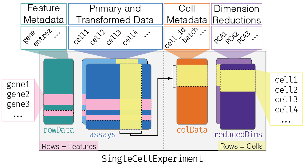
SingleCellExperiment

Load Dataset into R

We next use the read10xCounts function from the DropletUtils package to load the count matrix. This function automatically identifies the count matrix file from CellRanger’s output and reads it in as a SingleCellExperiment object.

fname <- file.path("untar_path", "pbmc4k/raw_gene_bc_matrices/GRCh38")
sce.pbmc <- read10xCounts(fname, col.names = TRUE)

With the data loaded, we can inspect the SCE object to see what information it contains.

sce.pbmc

class: SingleCellExperiment 
dim: 33694 737280 
metadata(1): Samples
assays(1): counts
rownames(33694): ENSG00000243485 ENSG00000237613 ... ENSG00000277475
  ENSG00000268674
rowData names(2): ID Symbol
colnames(737280): AAACCTGAGAAACCAT-1 AAACCTGAGAAACCGC-1 ...
  TTTGTCATCTTTAGTC-1 TTTGTCATCTTTCCTC-1
colData names(2): Sample Barcode
reducedDimNames(0):
altExpNames(0):

Questions:

• How many cells are in the SCE object? How many genes?

Removing empty droplets from unfiltered datasets

Droplet-based scRNA-seq methods like 10x increase the throughput of single-cell transcriptomics studies. However, one drawback to droplet-based sequencing is that some of the droplets will not contain a cell and will need to be filtered out computationally. This would be an easy task if empty droplets were truly empty, but in reality these droplets contain “ambient” RNA (free transcripts present in the cell suspension solution that are either actively secreted by cells or released upon cell lysis). These ambient RNAs serve as the base material for reverse transcription and scRNA-seq library preparation, resulting in non-zero counts for cell-less droplets/barcodes.

We can generate a knee plot to visualize the library sizes (i.e. total counts) for each barcode in the dataset. In this plot, high quality barcodes are located on the left and the “knee” represents the inflection point, where to the right barcodes have relatively low counts and may represent empty droplets.

bcrank <- barcodeRanks(counts(sce.pbmc))

# Only showing unique points for plotting speed.
uniq <- !duplicated(bcrank$rank)
plot(bcrank$rank[uniq], bcrank$total[uniq], log="xy",
    xlab="Rank", ylab="Total UMI count", cex.lab=1.2)

abline(h=metadata(bcrank)$inflection, col="darkgreen", lty=2)
abline(h=metadata(bcrank)$knee, col="dodgerblue", lty=2)

legend("bottomleft", legend=c("Inflection", "Knee"), 
        col=c("darkgreen", "dodgerblue"), lty=2, cex=1.2)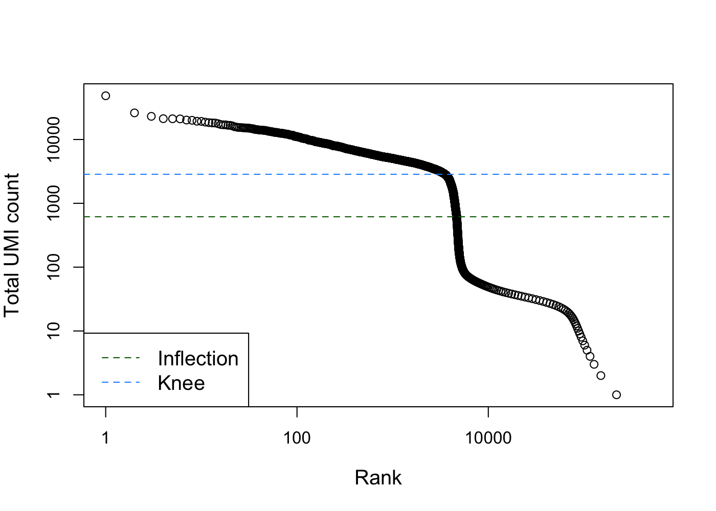

Past versions of knee_plot-1.png

Version	Author	Date
8cdfd4d	Davis McCarthy	2021-06-29

# Total UMI count for each barcode in the PBMC dataset,
# plotted against its rank (in decreasing order of total counts). 
# The inferred locations of the inflection and knee points are also shown.

Filtering just by library size may result in eliminating barcodes that contained cells with naturally low expression levels. Luckily, more accurate methods have been developed to filter out cell-less barcodes from droplet-based data. Here we use the emptyDrops method from the DropletUtils package, which estimates the profile of the ambient RNA pool and then tests each barcode for deviations from this profile [@Lun2019-tg].

set.seed(100)
e.out <- emptyDrops(counts(sce.pbmc))
sce.pbmc <- sce.pbmc[,which(e.out$FDR <= 0.001)]
unfiltered <- sce.pbmc
sce.pbmc

class: SingleCellExperiment 
dim: 33694 4300 
metadata(1): Samples
assays(1): counts
rownames(33694): ENSG00000243485 ENSG00000237613 ... ENSG00000277475
  ENSG00000268674
rowData names(2): ID Symbol
colnames(4300): AAACCTGAGAAGGCCT-1 AAACCTGAGACAGACC-1 ...
  TTTGTCAGTTAAGACA-1 TTTGTCATCCCAAGAT-1
colData names(2): Sample Barcode
reducedDimNames(0):
altExpNames(0):

Questions:

• How many cells are in the SCE object after filtering out empty barcodes?

Annotate genes

Let’s first add row names to rowData and we are going to use gene symbols as the row names. We have to ensure the row name for each gene is unique using the uniquifyFeatureNames function from scater. It will find the duplicated Symbols (some Ensembl IDs share the same gene symbol) and add Ensemble ID as prefix for them so that the rownames are unique.

The PBMC SCE object has the Ensembl ID and the gene symbol for each gene in the rowData. We can add additional annotation information (e.g. chromosome origin) using the annotation database package EnsDb.Hsapiens.v86. Then, to get additional annotations of these genes we can use the IDs as keys to retrieve the information from the database using the mapIds function.

rownames(sce.pbmc) <- uniquifyFeatureNames( ID = rowData(sce.pbmc)$ID, 
                                            names = rowData(sce.pbmc)$Symbol)

location <- mapIds(EnsDb.Hsapiens.v86, keys=rowData(sce.pbmc)$ID, 
    column="SEQNAME", keytype="GENEID")

head(location)

ENSG00000243485 ENSG00000237613 ENSG00000186092 ENSG00000238009 ENSG00000239945 
            "1"             "1"             "1"             "1"             "1" 
ENSG00000239906 
            "1" 

Quality control and data visualisation

Expression QC overview

Cell-level QC

With empty barcodes removed, we can now focus on filtering out low-quality cells (i.e. damaged or dying cells) which might interference with our downstream analysis. It’s common practice to filter cells based on low/high total counts, but we may also want to remove cells with fewer genes expressed. However, for heterogeneous cell populations, like PBMCs, this may remove cell types with naturally low RNA content. So here we will be more relaxed in our filtering and only remove cells with large fraction of read counts from mitochondrial genes. This metric is a proxy for cell damage, where a high proportion of mitochondrial genes would suggest that cytoplasmic mRNA leaked out through a broken membrane, leaving only the mitochondrial mRNAs still in place.

We first calculate QC metrics by perCellQCMetrics function from scater and then filter out the cells with outlying mitochondrial gene proportions.

stats <- perCellQCMetrics(sce.pbmc, subsets=list(Mito=which(location=="MT")))

high.mito <- isOutlier(stats$subsets_Mito_percent, type="higher")
colData(sce.pbmc) <- cbind(colData(sce.pbmc), stats)

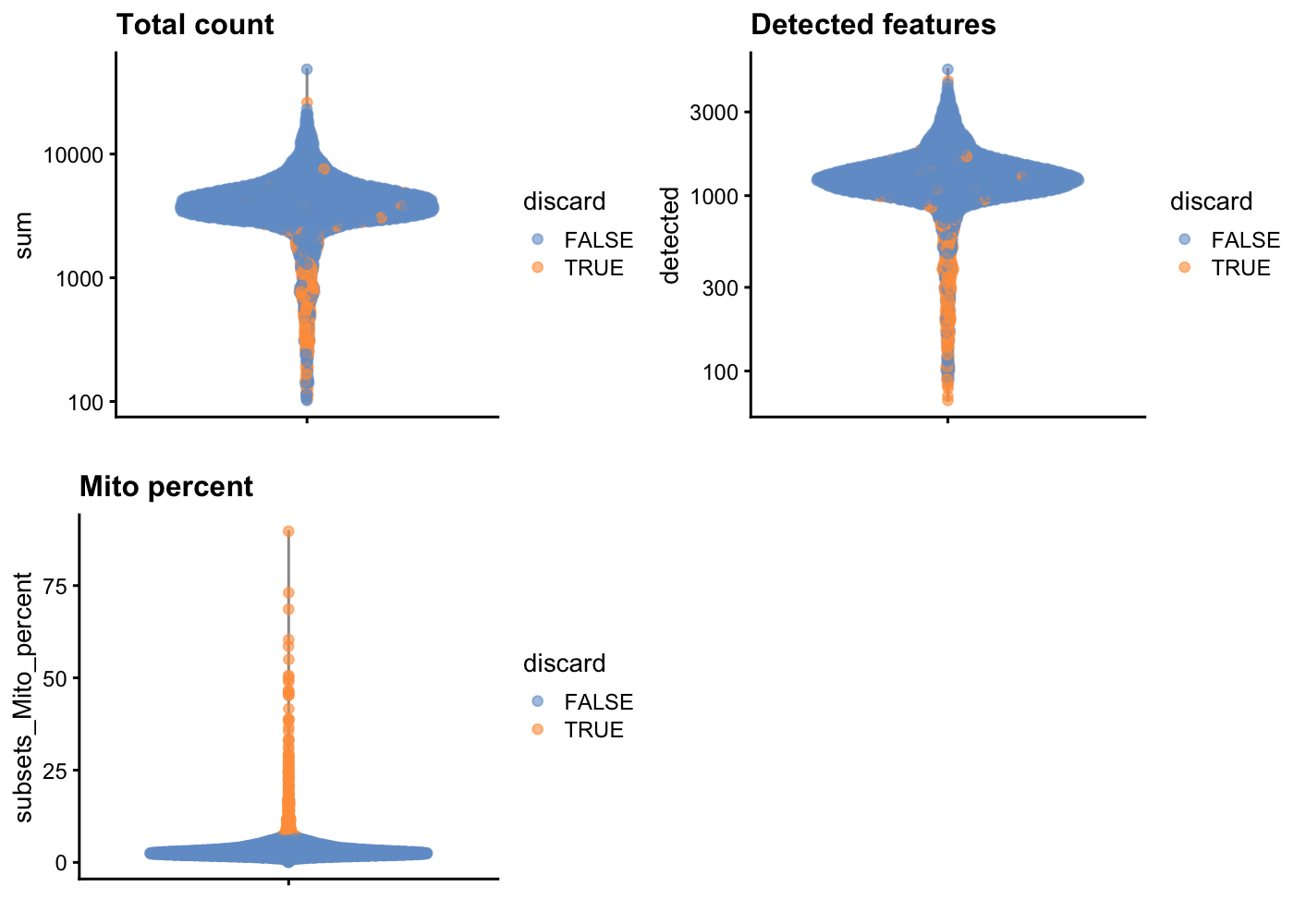
sce.pbmc <- sce.pbmc[,!high.mito]

As sanity check, we can look at the library size (i.e. total counts per cell) for cells that will remain after filtering and those that will be removed for having high mitochondrial mRNA proportions. As expected, the cells that will be filtered out (orange) tend to have lower library sizes, but not all cells with low library sizes are removed.

If a large proportion of cells will be removed, then it suggests that the QC metrics we are using for filtering might be correlated with some biological state.

colData(unfiltered) <- cbind(colData(unfiltered), stats)
unfiltered$discard <- high.mito

plotColData(unfiltered, y="sum", colour_by="discard") +
        scale_y_log10() + ggtitle("Total count")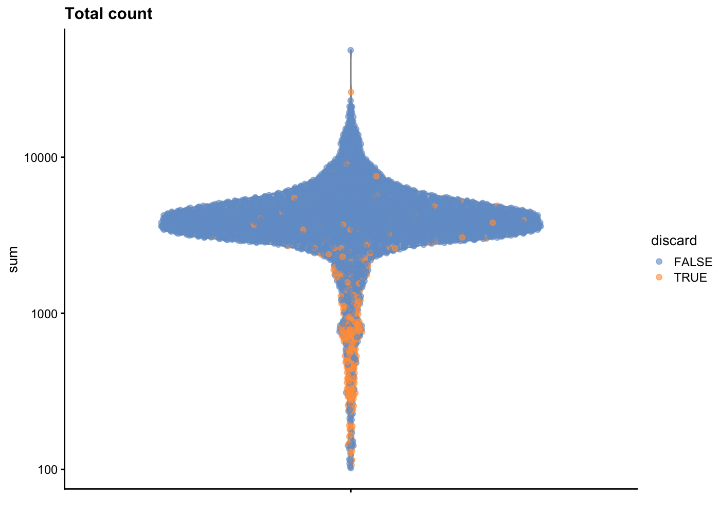

Past versions of plot_coldata-1.png

Version	Author	Date
8cdfd4d	Davis McCarthy	2021-06-29

In another view, we plot the subsets_Mito_percent against sum:

plotColData(unfiltered, x="sum", y="subsets_Mito_percent", colour_by="discard")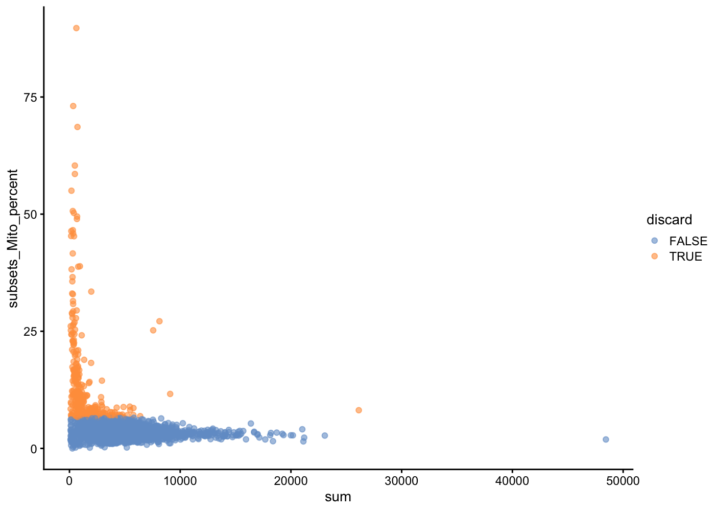

Past versions of plot_sum_mito-1.png

Version	Author	Date
8cdfd4d	Davis McCarthy	2021-06-29

The aim is to confirm that there are no cells with both large total counts and large mitochondrial counts, to ensure that we are not inadvertently removing high-quality cells that happen to be highly metabolically active (e.g., hepatocytes).

Points in the top-right corner might potentially correspond to metabolically active, undamaged cells.

Hands on exercises

—1. Try identifying outlier cells based on low/high total counts—-

—2. Why would be useful to filter out cells with higher total counts—

—3. Use plotColData to plot other useful cell-level QC metrics (e.g. number of detected features, subsets_Mito_detected) and colour by whether cells would be discarded.—

Hint: you may find the following code helpful.

gridExtra::grid.arrange(
    plotColData(unfiltered, y = "sum", colour_by = "discard") +
        scale_y_log10() + ggtitle("Total count"),
    plotColData(unfiltered, y = "detected", colour_by = "discard") +
        scale_y_log10() + ggtitle("Detected features"),
    plotColData(unfiltered, y = "subsets_Mito_percent",
        colour_by = "discard") + ggtitle("Mito percent"),
    ncol = 2
)

Past versions of hint-1.png

Version	Author	Date
8cdfd4d	Davis McCarthy	2021-06-29

Doublet detection

Another form of QC is detecting doublets: droplets which contain multiple cells. Methods to detect doublets use the idea that doublets will contain co-expressed pairs of genes that we would not normally expect to be co-expressed. Here we will use the scds package to detect doublets.

The scds contains two separate methods cxds(), a co-expression based approach, and bcds(), a binary classification approach to discriminate artificial doublets from original data. The package also implements a hybrid method, cxds_bcds_hybrid(). For details, please see the scds package documentation and the scds paper. Here, we demonstrate the use of the cxds_bcds_hybrid() approach.

library(scds)
sce.pbmc <- cxds_bcds_hybrid(sce.pbmc)

[17:41:22] WARNING: amalgamation/../src/learner.cc:1095: Starting in XGBoost 1.3.0, the default evaluation metric used with the objective 'binary:logistic' was changed from 'error' to 'logloss'. Explicitly set eval_metric if you'd like to restore the old behavior.

sce.pbmc$doublet_outlier <- isOutlier(sce.pbmc$hybrid_score, nmads = 5)
hist(sce.pbmc$hybrid_score) 
abline(v = min(sce.pbmc$hybrid_score[sce.pbmc$doublet_outlier]), col = "firebrick",
      lty = 2)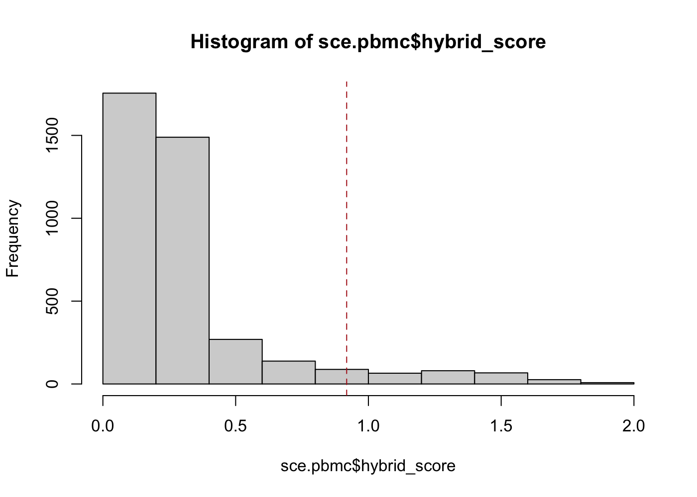

Past versions of doublet_detection-1.png

Version	Author	Date
752aaa3	Davis McCarthy	2021-07-05

table(sce.pbmc$doublet_outlier)

FALSE  TRUE 
 3703   282 

gridExtra::grid.arrange(
  plotColData(sce.pbmc, x = "total", y = "hybrid_score", colour_by = "detected"),
  plotColData(sce.pbmc, x = "total", y = "hybrid_score", colour_by = "doublet_outlier"),
  ncol = 2)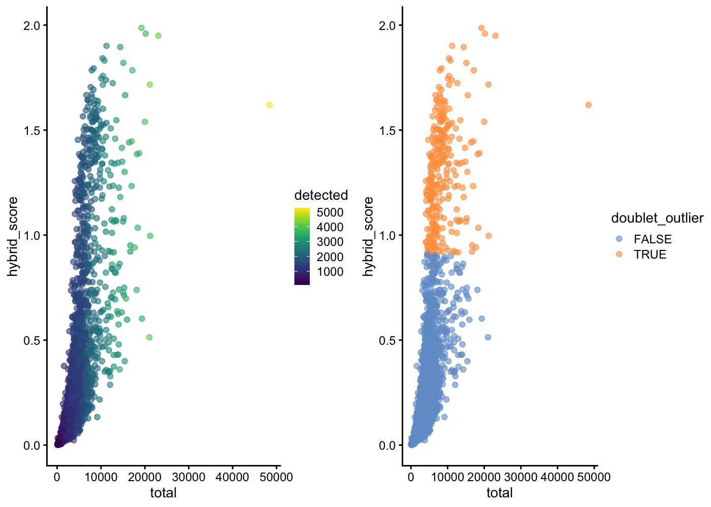

Past versions of doublet_detection-2.png

Version	Author	Date
752aaa3	Davis McCarthy	2021-07-05

In this example, scds's hybrid method finds 264 cells (barcodes) to be likely doublets if we define as outliers any cells with a hybrid_score more than 5 median absolute deviations away from the median. Even with a highly automated outlier detection method, there are choices for the analyst to make that will affect the final doublet detection results.

Please note that scds is by no means the only good or useful package available for expression based doublet detection for scRNA-seq data. It is also worth explicitly stating that this is a very challenging problem, and perfect accuracy in doublet detection is an unreasonable expectation

Gene QC

In addition to removing cells with poor quality, it is usually a good idea to exclude genes where we suspect that technical artefacts may have skewed the results. Moreover, inspection of the gene expression profiles may provide insights about how the experimental procedures could be improved.

It is often instructive to consider the number of reads consumed by the top 50 expressed genes.

plotHighestExprs(sce.pbmc[,sample(seq_len(ncol(sce.pbmc)), 200)], exprs_values = "counts")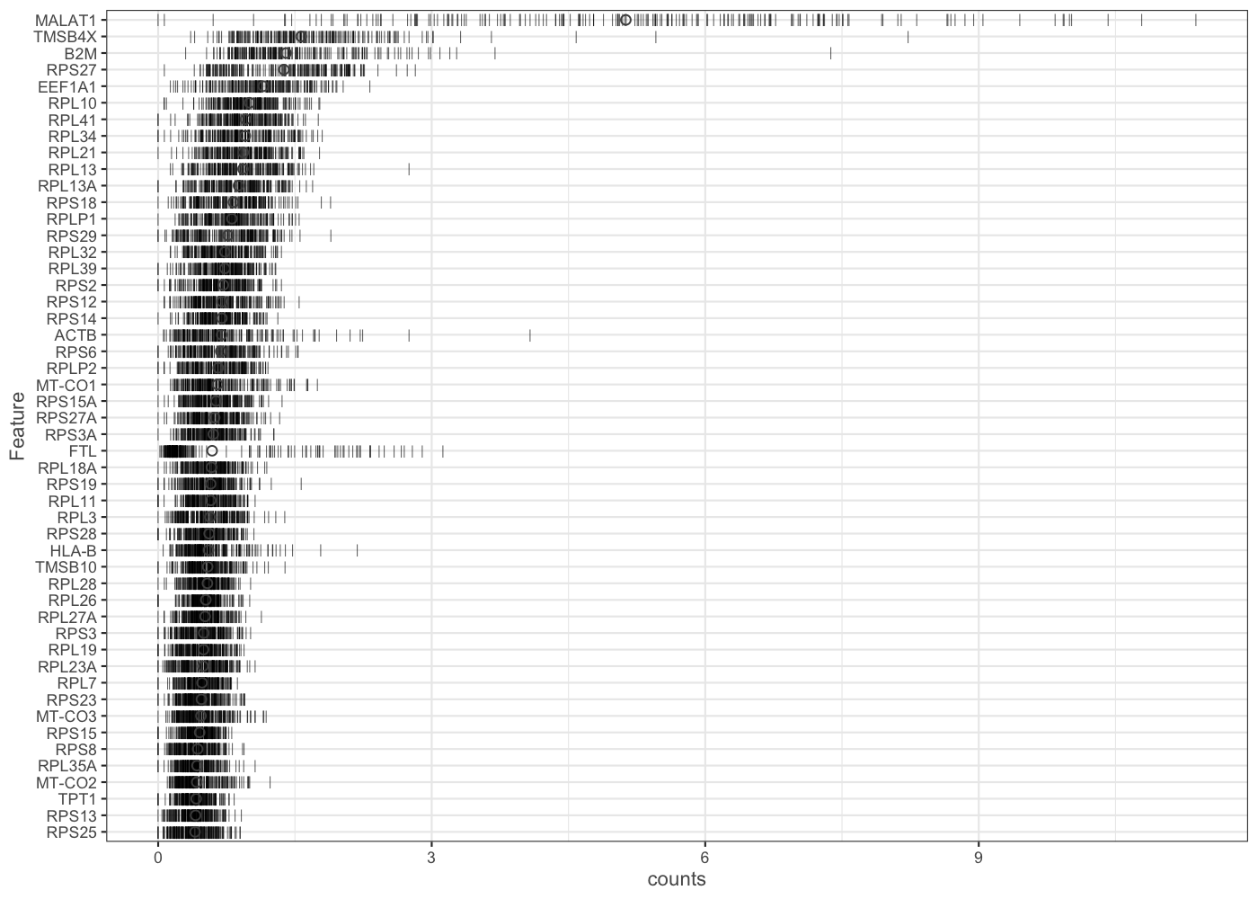

Past versions of plot_highest_genes-1.png

Version	Author	Date
752aaa3	Davis McCarthy	2021-07-05

[In this example we look just at expression in a random sample of 200 genes, for computational speed. If you have more time available you might like to replicate the plot using all cells from the sce.pbmc object.]

It is typically a good idea to remove genes whose expression level is considered “undetectable”. We define a gene as detectable if at least five cells contain more than 1 transcript from the gene. If we were considering read counts rather than UMI counts a reasonable threshold is to require at least five reads in at least two cells. However, in both cases the threshold strongly depends on the sequencing depth. It is important to keep in mind that genes must be filtered after cell filtering since some genes may only be detected in poor quality cells (note umi$use filter applied to the umi dataset).

keep_feature <- scater::nexprs(
  sce.pbmc, 
  byrow = TRUE, 
  detection_limit = 1
) >= 5

sce.pbmc <- sce.pbmc[keep_feature,]
table(keep_feature)

keep_feature
FALSE  TRUE 
25632  8062 

With this filter applied we retain about a quarter of the original genes - the others contain very little information so can be safely filtered out and drastically reduce computational time needed for subsequent analysis steps.

Data visualisation and exploratory data analysis

After having performed QC it is very important to visually explore the data to check for batch effects or other artifacts. To do this we can use a variety of visualisations. We will describe these in the Latent spaces section below.

Normalisation, confounders and batch correction

In this section, we will explore approaches to normalization, confounder identification and batch correction for scRNA-seq data.

Even in the absence of specific confounding factors, thoughtful normalization of scRNA-seq data is required. The raw count values are not directly comparable between cells, because in general the sequencing depth (number of reads obtained; often called library size) is very different across cells—orders-of-magnitude differences in sequencing depth are commonly observed between cells in an scRNA-seq dataset. If ignored, or not handled correctly, library size differences can be the dominant source of variation between single-cell gene expression profiles, obscuring the biological signal of interest. n Related to library size, differences in library composition can also cause problems when we are trying to compare expression profiles between cells. Normalization can and should also account for differences in library composition.

In addition to normalization, it is also useful to identify confounding factors so that they can be accounted for in downstream analyses. In many cases, “accounting” for confounding variables may involve incorporating them as variables in a particular statistical model (e.g. in a differential expression model). In other cases, it may be desirable to “regress out” (either in a literal or figurative sense) confounding factors—the challenge for scRNA-seq data is finding the right model and/or data transformation such that regressing out confounding factors would work as desired. We discuss this further below.

The issue of batch effects is just as important for scRNA-seq data as it is in other areas of genomics. Briefly, scRNA-seq and other ’omics assays are sensitive to minor differences in technical features of data generation. As such, even when assaying the same experimental or biological system, measurements taken at difference times and places or by different people will differ substantially. To make valid comparisons between cells, samples or groups, we first need to design our studies to be robust to batch effects and then we need to treat batch effects appropriately in our analyses.

In the following sections, we will explore simple size-factor normalizations correcting for library size and composition and also discuss a more recent, conceptually quite different, approach to tackling the problem of library size differences between cells.

Normalisation theory

Library size

Library sizes vary because scRNA-seq data is often sequenced on highly multiplexed platforms the total reads which are derived from each cell may differ substantially.

Most scRNA-seq platforms and/or quantification methods currently available produce count values as the “raw”, “observed”, gene expression values. For such count data, the library size must be corrected for as part of data normalization.

One popular strategy, borrowed and extended from the analysis of bulk RNA-seq data, is to multiply or divide each column of the expression matrix (in our setup columns correspond to cells) by a “normalization factor” which is an estimate of the library size relative to the other cells. Many methods to correct for library size have been developed for bulk RNA-seq and can be equally applied to scRNA-seq (eg. UQ, SF, CPM, RPKM, FPKM, TPM). In addition, single-cell specific size-factor normalization methods have been proposed to better handle the characteristics of scRNA-seq data (namely greater sparsity/proportion of zero counts). We will demonstrate use of the size-factor normalization method from the scran package in this chapter.

A conceptually different approach to normalization of scRNA-seq data was proposed earlier in 2019 by [@Hafemeister2019-rx]. The idea behind the sctransform approach is to fit a regularized negative binomial model to the raw count data, with library size as the only explanatory variable in the model. The residuals from this model can then be used as normalized and variance-stabilized expression values. We show the use of this method too in this chapter.

Some quantification methods (particularly those that quantify transcript-level expression, e.g. Salmon, kallisto) return transcripts-per-million values, TPM (instead of or in addition to count values), which effectively incorporate library size when determining gene expression estimates and thus do not require subsequent normalization for library size. However, TPM values may still be susceptible to library composition biases and so normalization may still be required.

Scaling or size-factor normalization methods

The normalization methods discussed in this section all involve dividing the counts for each cell by a constant value to account for library size and, in some cases, library composition. These methods will typically give (adjusted/normalized) counts-per-million (CPM) or transcripts-per-million (TPM) values.

Ideally, after applying one of these scaling/size-factor normalization methods, the CPM/TPM values produced are comparable across cells, with the effects of sequencing depth removed. However, even if this is true (i.e. the normalization has worked well), the CPM/TPM values do not have stable variance. Specifically, as the size of the values increases, so does the variance. This feature of the data (heteroskedacity, or asymmetric, heavy-tailed distributions) is problematic for statistical analysis methods that assume homoskedacity, that is that there is no relationship between the mean of expression values and their variance (i.e. just about anything that uses a Gaussian error model).

As such, we should apply a variance stabilizing transformation to these data so that we can use standard statistical methods like linear regression and PCA with confidence. Developing a thoroughly effective variance stabilizing transformation is a challenge, so almost universally a log transformation (typically log2) is applied to the CPM/TPM values (the logcounts slot in a SingleCellExperiment object is expected to contain (normalized) log2-scale CPM/TPM values). For high-depth cells and highly-expressed genes this transformation generally works well (as for bulk RNA-seq data), but, as we will discuss below, it often performs sub-optimally for (sparse) scRNA-seq data.

CPM

The simplest way to normalize this data is to convert it to counts per million (CPM) by dividing each column by its total then multiplying by 1,000,000. Note that spike-ins should be excluded from the calculation of total expression in order to correct for total cell RNA content, therefore we will only use endogenous genes. Example of a CPM function in R (using the scater package):

logcounts(sce.pbmc) <- log2(calculateCPM(sce.pbmc) + 1)

One potential drawback of CPM is if your sample contains genes that are both very highly expressed and differentially expressed across the cells. In this case, the total molecules in the cell may depend of whether such genes are on/off in the cell and normalizing by total molecules may hide the differential expression of those genes and/or falsely create differential expression for the remaining genes.

Note RPKM, FPKM and TPM are variants on CPM which further adjust counts by the length of the respective gene/transcript. TPM is usually a direct output of a transcript expression quantification method (e.g. Salmon, kallisto, etc).

To deal with this potentiality several other measures were devised.

RLE (SF)

The size factor (SF) was proposed and popularized by DESeq [@Anders2010-jr]. First the geometric mean of each gene across all cells is calculated. The size factor for each cell is the median across genes of the ratio of the expression to the gene’s geometric mean. A drawback to this method is that since it uses the geometric mean only genes with non-zero expression values across all cells can be used in its calculation, making it unadvisable for large low-depth scRNASeq experiments. edgeR & scater call this method RLE for “relative log expression” (to distinguish it from the many other size-factor normalization methods that now exist). Example of a SF function in R (from the edgeR package):

sizeFactors(sce.pbmc) <- edgeR::calcNormFactors(counts(sce.pbmc), method = "RLE")

UQ

The upperquartile (UQ) was proposed by [@Bullard2010-eb]. Here each column is divided by the 75% quantile of the counts for each library. Often the calculated quantile is scaled by the median across cells to keep the absolute level of expression relatively consistent. A drawback to this method is that for low-depth scRNASeq experiments the large number of undetected genes may result in the 75% quantile being zero (or close to it). This limitation can be overcome by generalizing the idea and using a higher quantile (eg. the 99% quantile is the default in scater) or by excluding zeros prior to calculating the 75% quantile. Example of a UQ function in R (again from the edgeR package):

sizeFactors(sce.pbmc) <- edgeR::calcNormFactors(counts(sce.pbmc), method = "upperquartile")

TMM

Another method is called TMM is the weighted trimmed mean of M-values (to the reference) proposed by [@Robinson2010-hz]. The M-values in question are the gene-wise log2-fold changes between individual cells. One cell is used as the reference then the M-values for each other cell is calculated compared to this reference. These values are then trimmed by removing the top and bottom ~30%, and the average of the remaining values is calculated by weighting them to account for the effect of the log scale on variance. Each non-reference cell is multiplied by the calculated factor. Two potential issues with this method are insufficient non-zero genes left after trimming, and the assumption that most genes are not differentially expressed.

sizeFactors(sce.pbmc) <- edgeR::calcNormFactors(counts(sce.pbmc), method = "TMM")

scran

scran package implements a variant on CPM size-factor normalization specialized for single-cell data [@L_Lun2016-pq]. Briefly this method deals with the problem of vary large numbers of zero values per cell by pooling cells together calculating a normalization factor (similar to TMM) for the sum of each pool. Since each cell is found in many different pools, cell-specific factors can be deconvoluted from the collection of pool-specific factors using linear algebra.

This method applies a “quick cluster” method to get rough clusters of cells to pool together to apply the strategy outlined above.

qclust <- quickCluster(sce.pbmc, min.size = 30)
sce.pbmc <- computeSumFactors(sce.pbmc, sizes = 15, clusters = qclust)

sctransform

The sctransform method is very different from the scaling/size-factor methods discussed above. In their paper, [@Hafemeister2019-rx] argue that the log-transformation of (normalized) CPM values does not stabilise the variance of expression values, particularly in the case of sparse(r) UMI-count data. Figure 1 of their paper (reproduced below) sets out this argument that strong relationships exist between gene expression and total cell UMI count, even after applying a scaled log-normalization method.

Reproduction of Figure 1 from Hafemeister and Satija (2019). 33,148 PBMC dataset from 10x genomics. A) Distribution of total UMI counts / cell (’sequencing depth’). B) We placed genesinto six groups, based on their average expression in the dataset. C) For each gene group, we examined the average relationship between observed counts and cell sequencing depth. We fit a smooth line for each gene individually and combined results based on the groupings in (B). Black line shows mean, colored region indicates interquartile range. D) Same as in (C), but showing scaled log-normalized values instead of UMI counts. Values were scaled (z-scored) so that a single y-axis range could be used. E) Relationship between gene variance and cell sequencing depth; Cells were placed into five equal-sized groups based on total UMI counts (group 1 has the greatest depth), and we calculated the total variance of each gene group within each bin. For effectively normalized data, each cell bin should contribute 20% to the variance of each gene group.

One effect of the failure of the scaled log-normalization to remove the relationship between total cell UMI count and expression is that dimension-reduction methods (especially PCA) applied to the log-normalized data can return reduced dimension spaces where, very often, the first dimension is highly correlated with total cell UMI count to total cell genes expressed. This effect is noted and discussed by [@William_Townes2019-wg].

The sctransform solution is to fit a negative binomial (NB) generalized linear model to the UMI counts for each gene, with an intercept term and a coefficient for library size (specifically using log10(total cell UMI count) as a covariate) as parameters in the model. The negative binomial model can account for much more variance in the observed count data than a simpler model like the Poisson can. To avoid overfitting the model to the data, the gene-wise intercept, library size and overdispersion parameters are regularized by fitting a loess (locally-linear smoothing method) to the per-gene estimates from the GLM.

Reproduction of Figure 2A from Hafemeister and Satija (2019). They fit NB regression models for each gene individually, and bootstrapped the process to measure uncertainty in the resulting parameter estimates. A) Model parameters for 16,809 genes for the NB regression model, plotted as a function of average gene abundance. The color of each point indicates a parameter uncertainty score as determined by bootstrapping (Methods). Pink line shows the regularized parameters obtained via kernel regression.

The regularized NB GLM is presented as an attractive middle ground between the (underfit) Poisson model and the (overfit) unregularized NB model. The Pearson residuals from the regularized NB GLM are used as “normalized” expression values for downstream analyses.

Reproduction of Figure 4 from Hafemeister and Satija (2019). A) For four genes, we show the relationship between cell sequencing depth and molecular counts. White points show the observed data. Background color represents the Pearson residual magnitude under three error models. For MALAT1 (does not vary across cell types) the Poisson error model does not account for overdispersion, and incorrectly infers significant residual variation (biological heterogeneity). For S100A9 (a CD14+ Monocyte marker) and CD74 (expressed in antigen-presenting cells) the non-regularized NB model overfits the data, and collapses biological heterogeneity. For PPBP (a Megakaryocyte marker) both non-regularized models wrongly fit a negative slope. B) Boxplot of Pearson residuals for models shown in A. X-axis range shown is limited to [-8, 25] for visual clarity.

The regularized NB GLM also provides a natural way to do feature selection (i.e. find informative genes) using the deviance of the fitted GLM for each gene. We discuss this further in the Variance modeling section.

We find the Pearson residuals from sctransform to be highly suitable as input to visualisation (dimension reduction) and clustering methods. For several other analyses (e.g. differential expression analyses), where statistical models designed for sparse count data are available, we prefer to use approaches that work with the “raw” count data. We are not yet sure how well sctransform performs on full-length transcript (i.e. non-UMI) count data.

Downsampling

A final way to correct for library size is to downsample the expression matrix so that each cell has approximately the same total number of molecules. The benefit of this method is that zero values will be introduced by the down sampling thus eliminating any biases due to differing numbers of detected genes. However, the major drawback is that the process is not deterministic so each time the downsampling is run the resulting expression matrix is slightly different. Thus, often analyses must be run on multiple downsamplings to ensure results are robust.

Downsampling to the depth of the cell with the lowest sequencing depth (that still passes QC) will typically discard much (most) of the information gathered in a (typically expensive) scRNA-seq experiment. We view this as a heavy price to pay for a normalization method that generally does not seem to outperform alternatives. Thus, we would not recommend downsampling as a normalization strategy for scRNA-seq data unless all alternatives have failed.

Effectiveness

To compare the efficiency of different normalization methods we will use visual inspection of PCA plots and calculation of cell-wise relative log expression via scater’s plotRLE() function. Namely, cells with many (few) reads have higher (lower) than median expression for most genes resulting in a positive (negative) RLE across the cell, whereas normalized cells have an RLE close to zero. Example of a RLE function in R:

scater::plotRLE(sce.pbmc, style = "minimal", colour_by = "detected")

Note The RLE, TMM, and UQ size-factor methods were developed for bulk RNA-seq data and, depending on the experimental context, may not be appropriate for single-cell RNA-seq data, as their underlying assumptions may be problematically violated.

Note The calcNormFactors function from the edgeR package implements several library size normalization methods making it easy to apply any of these methods to our data.

Note edgeR makes extra adjustments to some of the normalization methods which may result in somewhat different results than if the original methods are followed exactly, e.g. edgeR’s and scater’s “RLE” method which is based on the “size factor” used by DESeq may give different results to the estimateSizeFactorsForMatrix method in the DESeq/DESeq2 packages. In addition, some (earlier) versions of edgeR will not calculate the normalization factors correctly unless lib.size is set at 1 for all cells.

Note For CPM normalisation we use scater’s calculateCPM() function. For RLE, UQ and TMM we used to use scater’s normaliseExprs() function, but it was deprecated and has been removed from the package). For scran we use the scran package to calculate size factors (it also operates on SingleCellExperiment class) and scater’s normalize() to normalise the data. All these normalization functions save the results to the logcounts slot of the SCE object.

Normalisation in action (UMI data)

Here, we demonstrate normalisation applied to a UMI dataset. The same principles and approaches generally also work well for read-count data.

Normalisation aims to remove systematic or technical differences (for example, from systematic differences in sequencing coverage across libraries or cells) among cells and samples so they do not interfere with comparisons of the expression profiles.

We are going to use a normalisation method named Normalisation by Deconvolution from scran, one of the library-size scaling methods discussed above that was developed to account for the sparsity challenges present with scRNA-seq data.

It is a scaling-based procedure that involves dividing all counts for each cell by a cell-specific scaling factor, often called a “size factor”. The size factor for each cell represents the estimate of the relative bias in that cell, so division of its counts by its size factor should remove that bias.

Adapted from bulk RNAseq analysis, we assume the majority of genes between two cells are non-DE (not differential expressed) and the difference among the non-DE genes are used to represent bias that is used to compute an appropriate size factor for its removal.

Given the characteristics of low-counts in single cell dataset, we first pool counts of cells together and estimate a pool-based size factor. The size factor for the pool can be written as a linear equation of the size factors for the cells within the pool. Repeating this process for multiple pools will yield a linear system that can be solved to obtain the size factors for the individual cells, hence deconvolved.

In addition, to avoid pooling too distinct cells together, we first do a quick clustering on the cells, and the normalisation (cell-pooling and deconvolution) is done for each cell cluster separately. [@Lun2016-ta].

After calculation of the size factors we apply a log transformation to the counts. This transformation is of the form:

\[ \log(\frac{y_{i j}}{s_i} + 1) \]

where \(y_ij\) is the observed count for gene \(j\) in cell \(i\) and \(s_i\) is the calculated size factor for cell \(i\). the division by the size factor removes the scaling bias, as described above, while the \(\log\) transformation helps to stabilize the variance of the counts making downstream visualisation and methods such as PCA more effective. The addition of 1 (sometimes called a pseudocount) is needed as \(\log(0)\) is \(-\infty\) - a value not useful for data analysis.

Take a look at an RLE plot applied to the raw count data for this PBMC data:

scater::plotRLE(sce.pbmc[, order(sce.pbmc$detected)], style = "minimal", 
                colour_by = "detected", exprs_values = "counts")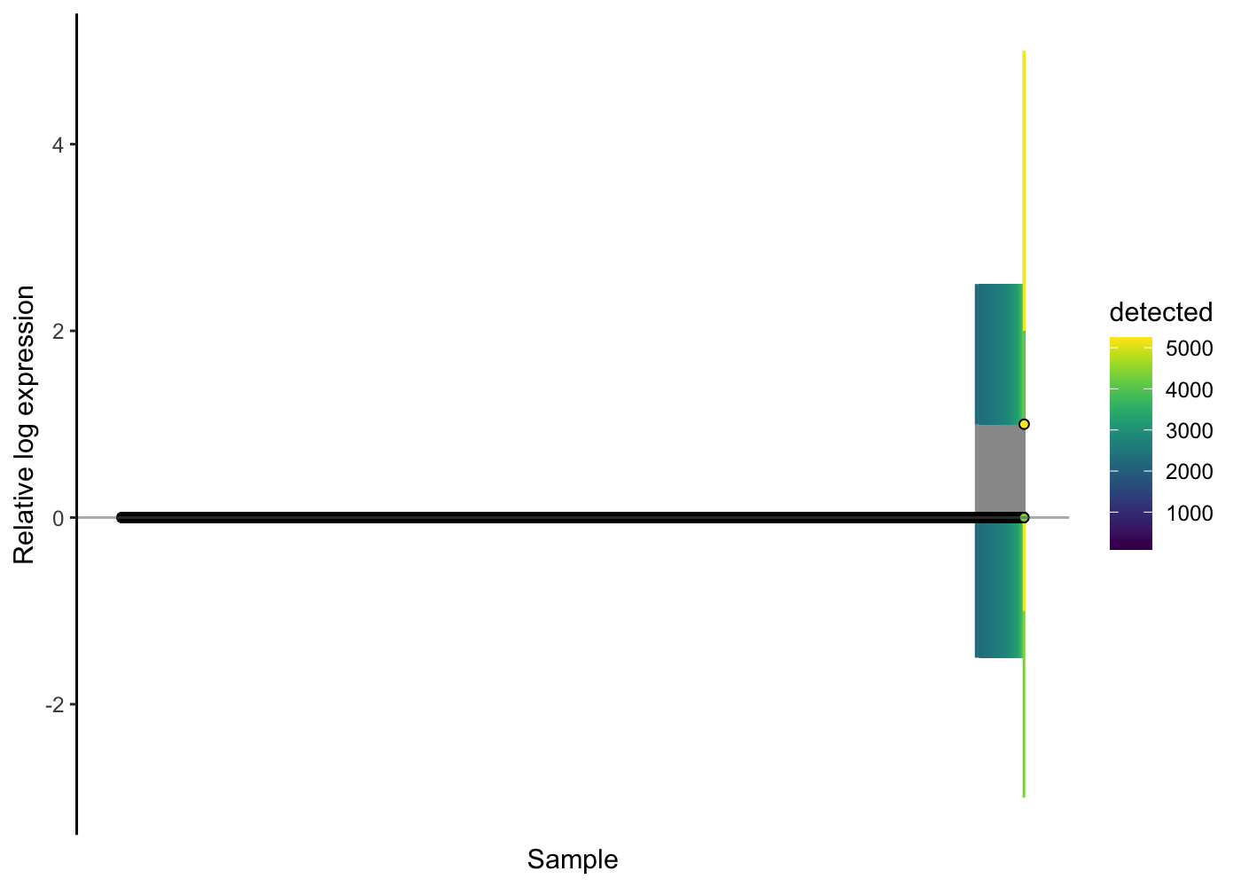

Past versions of rle-raw-counts-1.png

Version	Author	Date
9ec2636	Davis McCarthy	2021-07-05

We observe here that the majority of cells show no problems on the RLE plot, but for the cells with more than about 2500 genes with detected expression (about 130 cells here) their relative log expression for many genes is greater than two - a sign that better normalisation is required.

library(scran)
set.seed(1000)
clusters <- quickCluster(sce.pbmc)
sce.pbmc <- computeSumFactors(sce.pbmc, cluster = clusters)
## normalise using size factor and log-transform them
sce.pbmc <- logNormCounts(sce.pbmc)

We see that the scran deconvolution size factors are strongly correlated with library sizes for cells, as one would expect.

plot(librarySizeFactors(sce.pbmc), sizeFactors(sce.pbmc), pch = 16,
    xlab = "Library size factors", ylab = "Deconvolution factors", 
    log = "xy")
abline(a = 0, b = 1)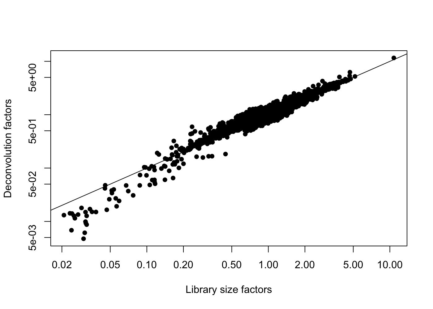

Past versions of plot_size_factors-1.png

Version	Author	Date
9ec2636	Davis McCarthy	2021-07-05
8cdfd4d	Davis McCarthy	2021-06-29

We can check the effectiveness of the normalisation method by using the RLE plot again.

scater::plotRLE(sce.pbmc[, order(sce.pbmc$detected)], style = "minimal", 
                colour_by = "detected", exprs_values = "logcounts")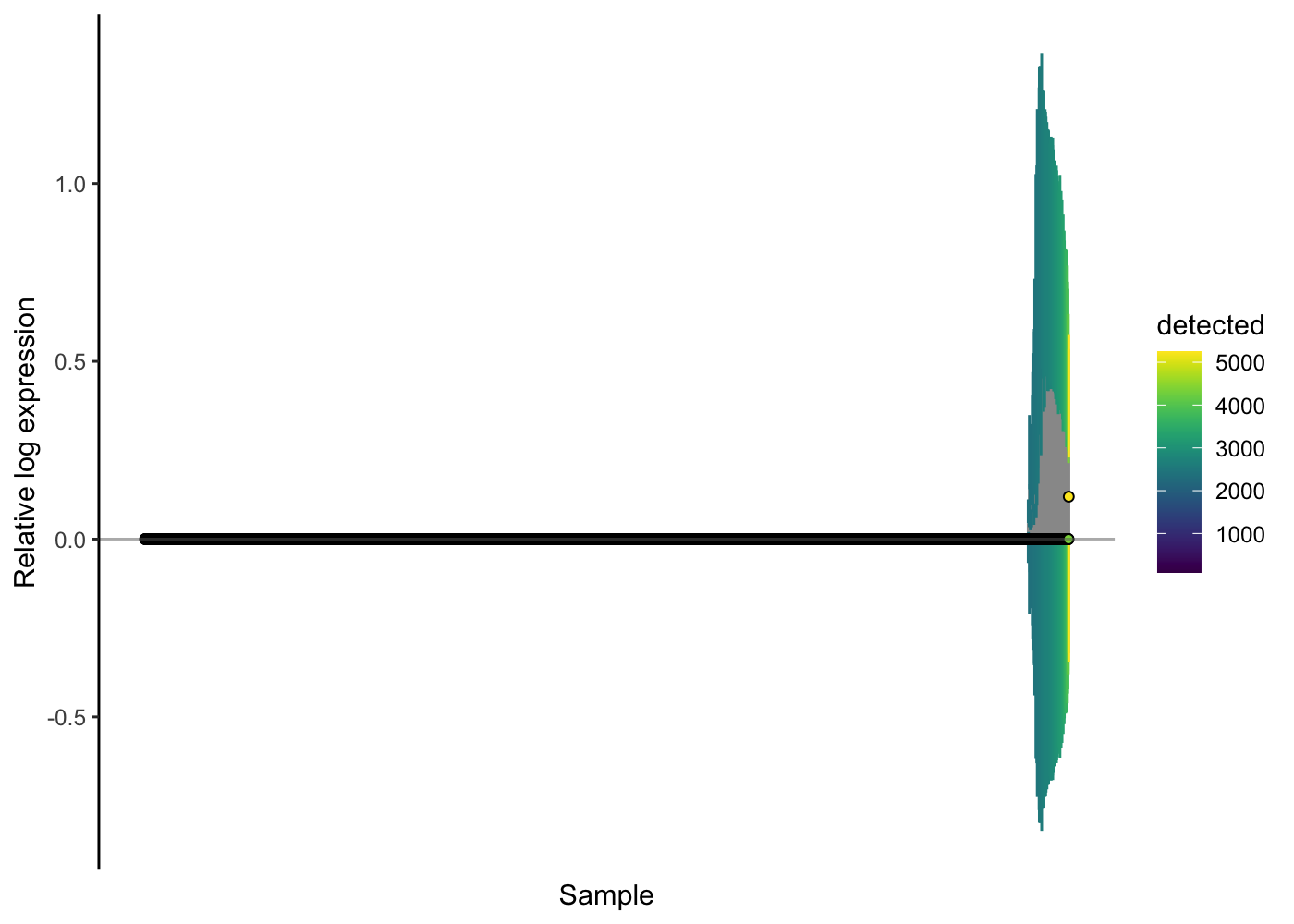

Past versions of rle-plots-norm-logcounts-1.png

Version	Author	Date
9ec2636	Davis McCarthy	2021-07-05

Here, the RLE plots show that the scran normalisation approach has improved the RLE of the high-genes-detected cells, but that there is still a notable difference there. We might wonder if any technical issues (e.g. doublets) are causing problems for the normalisation. Let’s use the colouring options in the RLE plot to investigate.

scater::plotRLE(sce.pbmc[, order(sce.pbmc$detected)], style = "minimal", 
                colour_by = "doublet_outlier", exprs_values = "logcounts")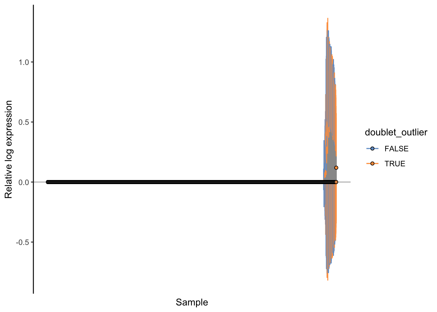

Past versions of rle-plots-norm-logcounts-doublets-1.png

Version	Author	Date
9ec2636	Davis McCarthy	2021-07-05

Indeed, it looks like probable doublet cells are enriched in these cells that are problematic with respect to normalisation. Let’s finally filter them out of our PBMC dataset, recompute the normalisation effects and check the outcome with an RLE plot.

set.seed(1000)
sce.pbmc <- sce.pbmc[, !sce.pbmc$doublet_outlier]
clusters <- quickCluster(sce.pbmc)
sce.pbmc <- computeSumFactors(sce.pbmc, cluster = clusters)
## normalise using size factor and log-transform them
sce.pbmc <- logNormCounts(sce.pbmc)
scater::plotRLE(sce.pbmc[, order(sce.pbmc$detected)], style = "minimal", 
                colour_by = "detected", exprs_values = "logcounts")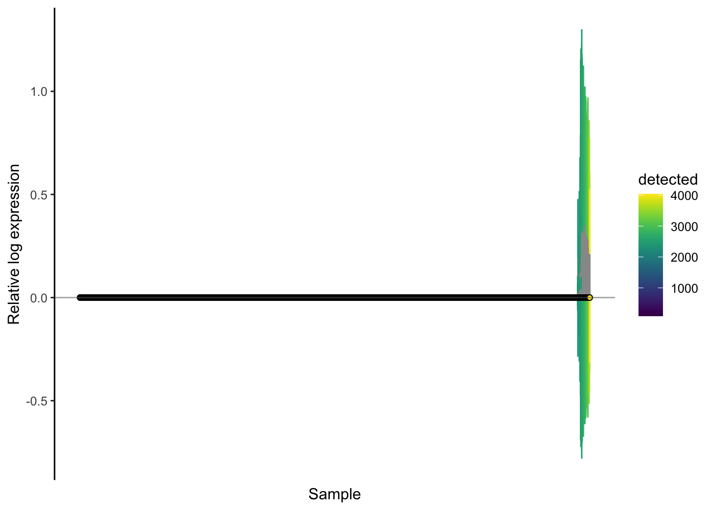

Past versions of size_factor_normalisation-no-doublets-1.png

Version	Author	Date
9ec2636	Davis McCarthy	2021-07-05

In this dataset, removing those probable doublets certainly helps. There are still osme cells that show differences in the RLE plot - one could consider filtering out such cells as “failures” of the normalisation procedure, but that is not routinely done and we will not filter them out for this analysis workflow.

ADVANCED EXERCISE: Alternative normalisation method

Recently, more sophisticated normalisation methods have been developed, for example sctransform [@Hafemeister2019-zh], as mentioned above.

If you are feeling confident with the normalisation approach described above, try applying sctransform normalisation to this dataset (and check its effectiveness), following the instructions in the sctransform package documentation and vignettes.

Variance modeling and feature selection

In this step, we would like to select the features/genes that represent the biological differences among cells while removing noise by other genes. We could simply select the genes with larger variance across the cell population based on the assumption that the most variable genes represent the biological differences rather than just technical noise.

The simplest approach to find such genes is to compute the variance of the log-normalised gene expression values for each gene across all cells. However, the variance of a gene in single-cell RNAseq dataset has a relationship with its mean. log-transformation does not achieve perfect variance stabilisation, which means that the variance of a gene is often driven more by its abundance than its biological heterogeneity.

To deal with this effect, we fit a trend to the variance with respect to the gene’s abundance across all genes to model the mean-variance relationship:

set.seed(1001)
dec.pbmc <- modelGeneVarByPoisson(sce.pbmc)

The trend is fitted on simulated Poisson count-derived variances with assumption that the technical component is Poisson-distributed and most genes do not exhibit large biological variability.

plot(dec.pbmc$mean, dec.pbmc$total, pch = 16, cex = 0.5,
    xlab = "Mean of log-expression", ylab = "Variance of log-expression")

curfit <- metadata(dec.pbmc)
curve(curfit$trend(x), col = 'dodgerblue', add = TRUE, lwd = 2)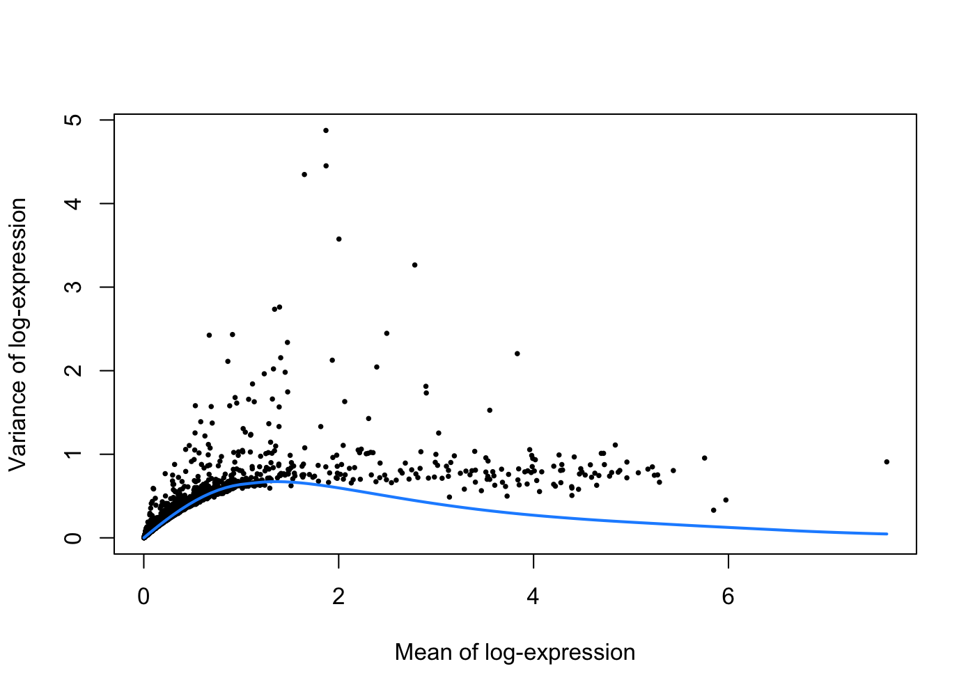

Past versions of plot_modelled_variance-1.png

Version	Author	Date
9ec2636	Davis McCarthy	2021-07-05
8cdfd4d	Davis McCarthy	2021-06-29

Under this assumption, our trend represents an estimate of the technical noise as a function of abundance. The total variance can then be decomposed into technical and biological components.

We can then get the list of highly variable genes after variance decomposition:

top.pbmc <- getTopHVGs(dec.pbmc, prop = 0.1)

About the number of genes to keep, if we believe no more than 5% of genes are differentially expressed across all the cells, we can set the prop to be 5%. In a more heterogeneous cell population, we would raise that number. Here we are using top 10%.

Note that the selection of the number of genes to keep is actually quite arbitrary. It is recommended to simply pick a value and go ahead with the downstream analysis but with the intention of testing other parameters if needed.

Latent spaces

Dimensionality reduction and visualisation

Now we have selected the highly variable genes, we can use these genes’ information to reveal cell population structures in a constructed lower dimensional space. Working with this lower dimensional representation allows for easier exploration and reduces the computational burden of downstream analyses, like clustering. It also helps to reduce noise by averaging information across multiple genes to reveal the structure of the data more precisely.

We first do a PCA (Principal Components Analysis) transformation. By definition, the top PCs capture the dominant factors of heterogeneity in the data set. Thus, we can perform dimensionality reduction by only keeping the top PCs for downstream analyses. The denoisePCA function will automatically choose the number of PCs to keep, using the information returned by the variance decomposition step to remove principal components corresponding to technical noise.

set.seed(10000)
## This function performs a principal components analysis to eliminate random 
## technical noise in the data.
sce.pbmc <- denoisePCA(sce.pbmc, subset.row = top.pbmc, technical = dec.pbmc)

sce.pbmc

class: SingleCellExperiment 
dim: 8062 3703 
metadata(1): Samples
assays(2): counts logcounts
rownames(8062): FO538757.2 AP006222.2 ... MT-CYB AL592183.1
rowData names(2): ID Symbol
colnames(3703): AAACCTGAGAAGGCCT-1 AAACCTGAGACAGACC-1 ...
  TTTGTCAGTTAAGACA-1 TTTGTCATCCCAAGAT-1
colData names(13): Sample Barcode ... doublet_outlier sizeFactor
reducedDimNames(1): PCA
altExpNames(0):

reducedDims(sce.pbmc)$PCA[1:5,]

                          PC1        PC2         PC3         PC4         PC5
AAACCTGAGAAGGCCT-1 -15.978700  2.3239565   0.9460592  0.01869805  3.76207846
AAACCTGAGACAGACC-1 -14.089896  7.7454934   4.9033006  0.25969024  0.08273299
AAACCTGAGGCATGGT-1   8.613559  1.3523423   3.8476151  2.03690624  2.95844623
AAACCTGCAAGGTTCT-1   7.816070 -0.6728106   2.6274823  0.92536303 -0.54936785
AAACCTGGTACATCCA-1   2.607899  4.2290679 -11.2991768 -0.68804669  2.10735348
                         PC6       PC7
AAACCTGAGAAGGCCT-1  1.102911 -1.227991
AAACCTGAGACAGACC-1 -0.786055 -2.907591
AAACCTGAGGCATGGT-1  1.037112  2.417100
AAACCTGCAAGGTTCT-1  1.168544 -1.145958
AAACCTGGTACATCCA-1  0.260318 -1.187410

tSNE (t-stochastic neighbor embedding) is a popular dimensionality reduction methods for visualising single-cell dataset with functions to run them available in scater. They attempt to find a low-dimensional representation of the data that preserves the distances between each point and its neighbours in the high-dimensional space.

In addition, UMAP (uniform manifold approximation and projection) which is roughly similar to tSNE, is also gaining popularity. They are ways to “visualise” the structure in the dataset and generate nice plots, but shouldn’t be regarded as the real clustering structure.

We actually instruct the function to perform the t-SNE calculations on the top PCs to use the data compaction and noise removal provided by the PCA.

set.seed(10000)
sce.pbmc <- runTSNE(sce.pbmc, dimred = "PCA")

Visualising column data or plotting gene expression in tSNE plot:

plotTSNE(sce.pbmc, colour_by = "detected")

Past versions of tsne_plot-1.png

Version	Author	Date
9ec2636	Davis McCarthy	2021-07-05
752aaa3	Davis McCarthy	2021-07-05

plotTSNE(sce.pbmc, colour_by = "CD14")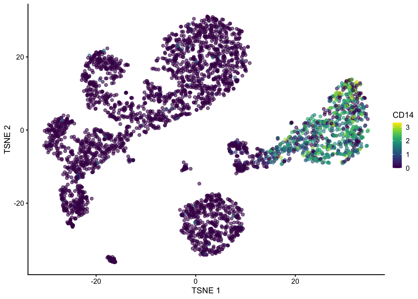

Past versions of tsne_plot-2.png

Version	Author	Date
9ec2636	Davis McCarthy	2021-07-05
752aaa3	Davis McCarthy	2021-07-05

Hexbin plot for overcoming overplotting

Notice that in the 2D plots of single cells, sometimes it can get really “crowded”, especially when the number of cells being plotted is large, and it runs into a over-plotting issue where cells are two close overlaying/blocking To deal with that, we can use the hexbin plots [@Freytag2020-us].

The schex package strategies for binning the observed cells into hexagonal cells. Plotting summarized information of all cells in their respective hexagonal cells presents information without obstructions.

We use the plot_hexbin_feature to plot the feature expression of single cells in bivariate hexagonal cells. These plots are extremely useful both for QC and biological investigations of the data (see plots below for doublet outlier status, mean number of total counts per cell and median expression of CD14).

pbmc_hex <- schex::make_hexbin(sce.pbmc, 100, dimension_reduction = "TSNE")

plot_hexbin_meta(pbmc_hex, col = "total", action = "mean") +
  ggtitle("Mean total number of counts per cell")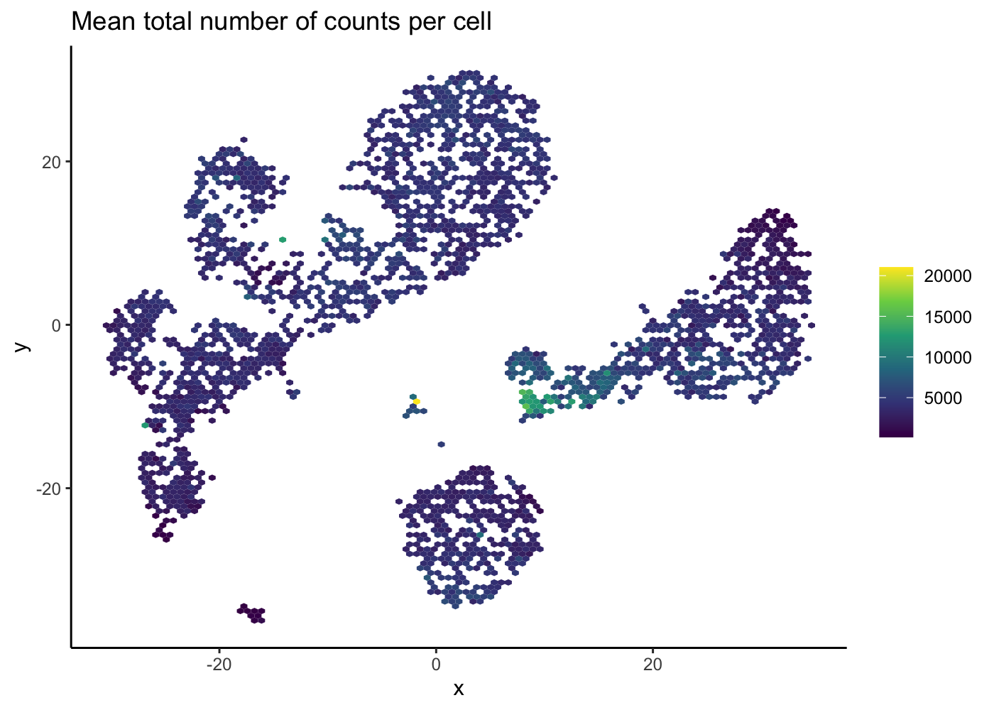

Past versions of hexgonplot-1.png

Version	Author	Date
9ec2636	Davis McCarthy	2021-07-05
752aaa3	Davis McCarthy	2021-07-05
8cdfd4d	Davis McCarthy	2021-06-29

plot_hexbin_feature(pbmc_hex,feature = "CD14",
                    type = "logcounts",
                    action = "median")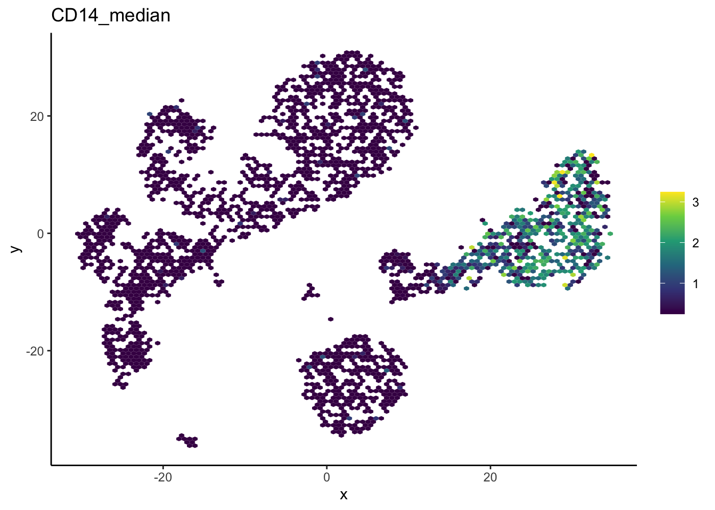

Past versions of hexgonplot-2.png

Version	Author	Date
9ec2636	Davis McCarthy	2021-07-05
752aaa3	Davis McCarthy	2021-07-05
8cdfd4d	Davis McCarthy	2021-06-29

Hands-on practice

—run UMAP and plot—-

—Plot the hexbin plot for UMAP dims—

Matrix factorisation and factor analysis

Another method for understanding single cell data through ‘reduction’ is matrix factorization and factor analysis. The key concept of factor analysis is that the original data are associated with some underlying unobserved variables: the latent factor. Hopefully. these latent factor are biologically meaningful, for example in single cell data a factor could correspond to a specific regulatory process. Research into factor analysis and matrix factorization is still ongoing but one leading method is Slalom which aims to make the latent factors more interpretable by enforcing sparsity constraints.

Autoencoders

The scVI paper can be credited with introducing and raising the profile of variational autoencoders - a relatively recent method from machine learning - for single-cell analysis. Variational autoencoders also use the idea of a latent space to understand structure in a dataset. Unlike more “traditional” matrix factorisation approaches, however, they use neural networks to compress information and can take advantage of gradient descent and GPU acceleration to scale to very large datasets. Since the publication of scVI, at least 40 methods have been proposed with twists on autoencoders; many of them provide excellent utility for data analysis, but a comprehensive survey is beyond the scope of what we can provide here. The scvi-tools webpage is now a great resource for related probabilistic methods for single-cell data analysis available in both Python and R that can interact with Bioconductor and Seurat workflows. We don’t have the space to explore them here, but they are very much worth exploring.

Clustering

One of the most promising applications of scRNA-seq is de novo discovery and annotation of cell-types based on transcription profiles. We are going to use unsupervised clustering method, that is, we need to identify groups of cells based on the similarities of the transcriptomes without any prior knowledge of the labels.

In scRNA-seq analyses, shared K-nearest neighbour graph-based clustering is often applied. Each cell is represented in the graph as a node, and the first step is to find all the KNN (K-neareast neighbours) for each cell by comparing their pair-wise Euclidean distances. After that, the nodes are connected if they have at least one shared nearest neighbors, and weights are also added to the edges by how many shared neighbours they have.

shared nearest neighbour

Once the SNN graph is built, we can then use different algorithms to detect communities/clusters in the graph. Here we use the method called ‘walktrap’ from the igraph package which tries to detect densely connected communities in a graph via random walks.

g <- buildSNNGraph(sce.pbmc, k = 20, use.dimred = 'PCA')
clust <- igraph::cluster_walktrap(g)$membership
colLabels(sce.pbmc) <- factor(clust)
table(factor(clust))

  1   2   3   4   5   6   7   8   9  10  11  12 
554 162 508 139 447 212 877 524  76  30 129  45 

Questions

— Choose different values for k and observe how many clusters you get —

Clustree

The clustree package can be used to visualise the different clustering results in a tree structure. It helps to visualise how cells move as the clustering resolution changes.

Note, it looks very much like a hierarchical clustering result but it is not.

g <- buildSNNGraph(sce.pbmc, k = 3, use.dimred = 'PCA')
k3 <- igraph::cluster_walktrap(g)$membership
g <- buildSNNGraph(sce.pbmc, k = 5, use.dimred = 'PCA')
k5 <- igraph::cluster_walktrap(g)$membership
g <- buildSNNGraph(sce.pbmc, k = 8, use.dimred = 'PCA')
k8 <- igraph::cluster_walktrap(g)$membership
g <- buildSNNGraph(sce.pbmc, k = 10, use.dimred = 'PCA')
k10 <- igraph::cluster_walktrap(g)$membership
g <- buildSNNGraph(sce.pbmc, k = 20, use.dimred = 'PCA')
k20 <- igraph::cluster_walktrap(g)$membership
g <- buildSNNGraph(sce.pbmc, k = 50, use.dimred = 'PCA')
k50 <- igraph::cluster_walktrap(g)$membership
multipleKResults <- data.frame(k3, k5, k8, k10, k20, k50)
clustree(multipleKResults, prefix = "k", prop_filter = 0.05, layout = "tree")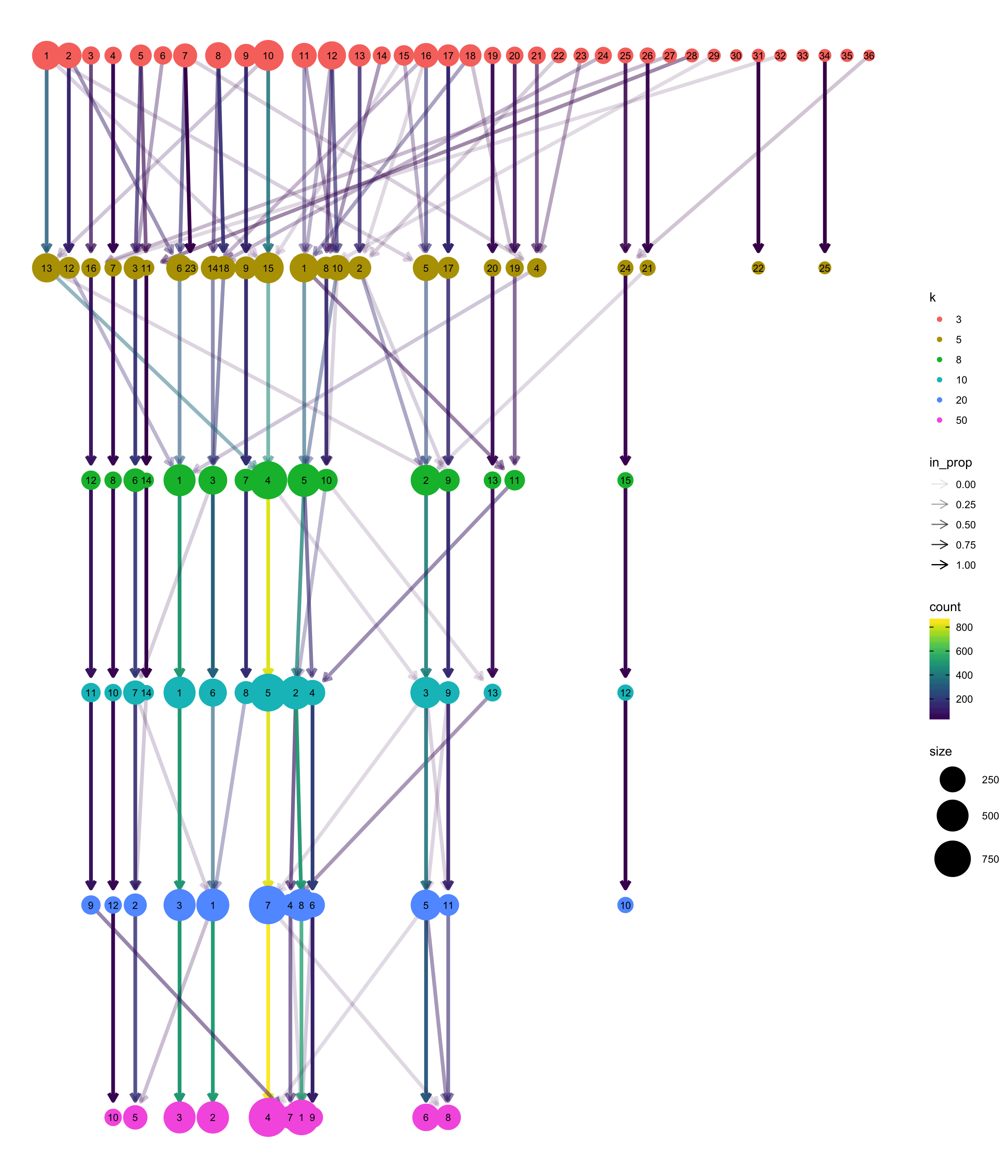

Past versions of hint,clustree-1.png

Version	Author	Date
9ec2636	Davis McCarthy	2021-07-05
8cdfd4d	Davis McCarthy	2021-06-29

Varying clustering resolutions is an important part of data exploration for scRNA-seq. It is challenging to find the best resolution, and you usually need to experiment with different parameters multiple times and to find the best result.

Plot Clusters

Plot clustering result in a t-SNE plot

plotTSNE(sce.pbmc, colour_by = "label")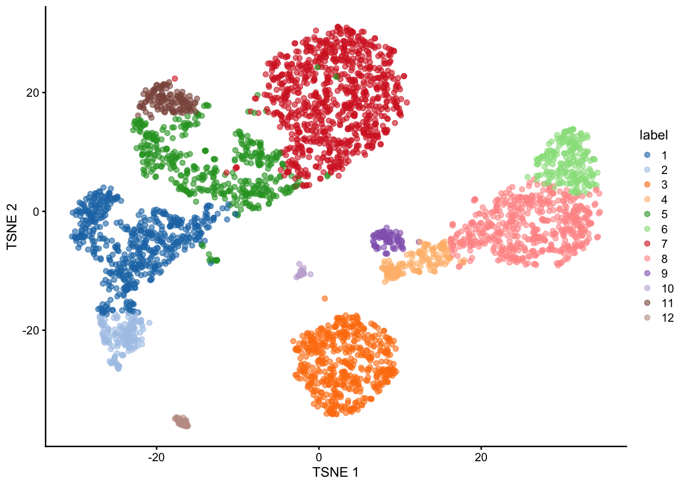

Past versions of plot_tsne_by_cluster-1.png

Version	Author	Date
9ec2636	Davis McCarthy	2021-07-05
8cdfd4d	Davis McCarthy	2021-06-29

Merging clusters

At this point, merging clusters to refine computationally-derived clusters into optimally biologically-relevant clusters is more art than science. In many settings it would be desirable to understand the hierarchical relationships between cell types and the annotations of cells to those cell types. At this point in time, we are not aware of computational methods that merge clusters in the way we might want. Readers interested in the topic, however, might be interested in following up with the MRtree method (Peng et al, NAR, 2021).

Marker detection and cluster annotation

To interpret our clustering results, we identify the genes that drive separation between clusters. These so-called ‘marker genes’ allow us to assign biological meaning to each cluster based by comparing the expression profiles of the marker genes to the expression profiles of previously identified cell types. We demonstrate this approach in the section “Manual” annotation.

An alternative way is to use some automatic annotation approach, see the “Automatic” annotation section.

“Manual” annotation

To identify the marker genes for each cluster we use the findMarkers() function from the scran package. The findMarkers() function uses pair-wise differential expression testing to identify marker genes. This means that, for each gene, it tests for differences in expression between the cluster of interest and each of the other clusters in the dataset seperately. By default, a t-test is used, but a binomial test or the Wilcoxon rank sum test are also implemented. In the code below we specify that we only want to idenfity genes which are "up" regulated in the cluster of interest. The returned results for one cluster (versus all of the remaining clusters) are combined into a single list and combined p-values are calculated. One can specifty the pval.type which determines how the DEGs are combined: any, return genes that are determined as up-regulated in any of the comparisons; all, return genes that are determined as up-regulated in all of the comparisons, some is a compromise between any and all.

markers <- findMarkers(sce.pbmc, pval.type = "some", direction = "up")

We examine the markers for cluster 7 and 14 in more detail.

marker.set <- markers[["7"]]
as.data.frame(marker.set[1:10,1:3])

             p.value           FDR summary.logFC
CD3G   1.574823e-150 1.269622e-146     0.9419999
LEF1   9.778578e-150 3.941745e-146     0.9508085
TRAC   2.225329e-135 5.980202e-132     2.2750028
CCR7   3.551170e-134 7.157384e-131     0.8449173
CD3D   3.947266e-100  6.364571e-97     1.7401943
CD27    4.733009e-93  6.359586e-90     0.9872458
MAL     1.270270e-87  1.462988e-84     0.5704063
IL7R    4.071572e-87  4.103127e-84     1.0106113
FLT3LG  4.071791e-81  3.647420e-78     0.6282038
LDHB    1.792951e-80  1.445477e-77     1.5969586

marker.set <- markers[["14"]]
as.data.frame(marker.set[1:10,1:3])

data frame with 0 columns and 0 rows

Question: What do you make of these detected marker genes? Do they look biologically relevant or just like noise?

Now given what we know about the cell types in PBMCs and the marker genes:

— Plot the expression of these marker genes by clusters, and identify what cells types each cluster has —

Markers	Cell Type
IL7R	CD4 T cells
CD14, LYZ	CD14+ Monocytes
MS4A1	B cells
CD8A	CD8 T cells
FCGR3A, MS4A7	FCGR3A+ Monocytes
GNLY, NKG7	NK cells
PPBP	Megakaryocytes
FCER1A, CST3	Dendritic Cells

plotExpression(sce.pbmc, features = c("CD14"), x = "label", colour_by = "label")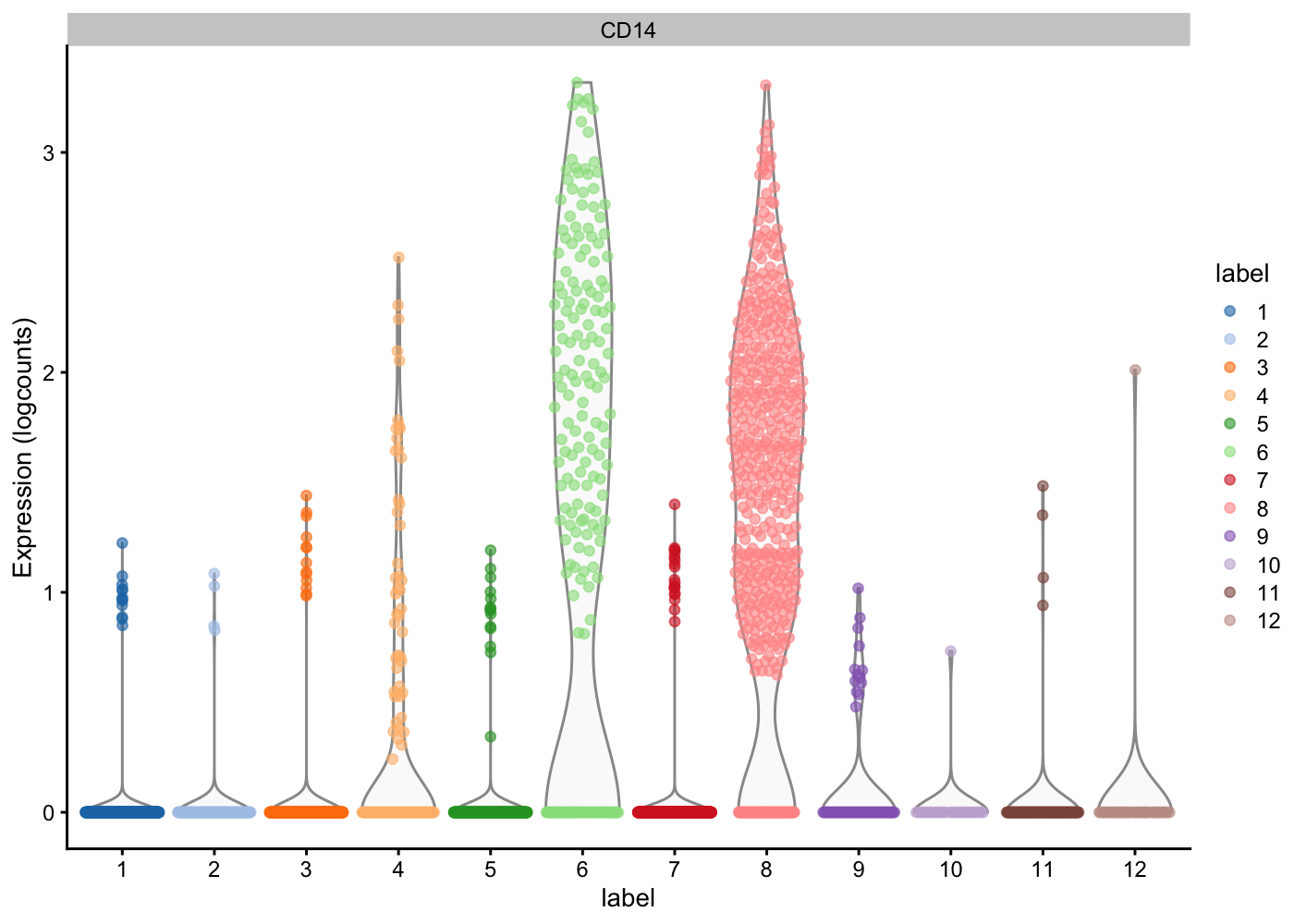

Past versions of unnamed-chunk-14-1.png

Version	Author	Date
9ec2636	Davis McCarthy	2021-07-05

“Automatic” annotation

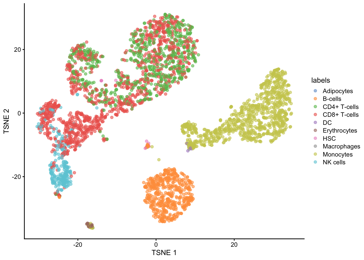
Intuitively, automatic annotation works by comparing the current dataset with previously annotated reference samples and finding the cell type of the most similar/correlated cells. SingleR method [@Aran2019-pw] provides one such option for cell type annotation. This method assigns labels to cells based on the reference samples with the highest Spearman rank correlations, using only the marker genes between pairs of labels to focus on the relevant differences between cell types. It also performs a fine-tuning step for each cell where the correlations are recomputed with just the marker genes for the top-scoring labels. This aims to resolve any ambiguity between those labels by removing noise from irrelevant markers for other labels.

library(SingleR)
ref <- celldex::BlueprintEncodeData()

snapshotDate(): 2020-10-27

see ?celldex and browseVignettes('celldex') for documentation

loading from cache

see ?celldex and browseVignettes('celldex') for documentation

loading from cache

pred <- SingleR(test = sce.pbmc, ref = ref, labels = ref$label.main)
table(pred$labels)

  Adipocytes      B-cells CD4+ T-cells CD8+ T-cells           DC Erythrocytes 
           1          525          748         1165            6           20 
         HSC  Macrophages    Monocytes     NK cells 
          16            3          974          245 

We can check the concordance of the SingleR annotations with our previous clustering result using a ‘confusion’ matrix.

table(pred$labels,sce.pbmc$label)

              
                 1   2   3   4   5   6   7   8   9  10  11  12
  Adipocytes     0   0   0   0   0   0   0   0   0   0   0   1
  B-cells        0   4 507   0   0   0   0   0   0  14   0   0
  CD4+ T-cells   1   6   0   0 183   0 486   0   0   0  72   0
  CD8+ T-cells 449  13   0   0 255   0 391   0   0   0  57   0
  DC             0   0   0   6   0   0   0   0   0   0   0   0
  Erythrocytes   0   1   0   0   0   0   0   0   0   0   0  19
  HSC            0   0   0   0   6   0   0   0   0  10   0   0
  Macrophages    0   0   0   2   0   0   0   0   0   1   0   0
  Monocytes      0   0   1 131   0 212   0 524  76   5   0  25
  NK cells     104 138   0   0   3   0   0   0   0   0   0   0

What do you think of the extent of (dis)agreement between our graph-based clustering of the cells and the SingleR reference-based cell-type annotation?

Cell type annotation plots

Now with the labels learned from SingleR methods, we can visualise them in a tSNE plot.

colData(sce.pbmc) <- cbind(colData(sce.pbmc),pred)
plotTSNE(sce.pbmc, colour_by = "labels")

Past versions of plot_singler_annotations-1.png

Version	Author	Date
9ec2636	Davis McCarthy	2021-07-05
8cdfd4d	Davis McCarthy	2021-06-29

Differential expression (DE) analysis

Introduction to DE analysis

Unlike analysing bulk RNA-seq data, where only one type of DE analysis is possible, many types of DE analysis can be performed on single cell data. Some different types DE analysis possible using single cell data are:

1. Comparing one cluster to all other clusters in a dataset
2. Comparing a specific pair of clusters (or groups of clusters) within a single dataset
3. Comparing the same cell type across samples in different conditions

Each of these different possible analyses require different methodologies. The first type of analysis is the same as finding marker genes (described above) and any marker gene methods which use differential expression testing can be used. A variety of methods are available for the second type of analysis. Recent benchmarking [@Soneson2018-hy] has suggested that edgeR, a differential expression method developed for bulk RNA-seq data performs well. Other options are MAST, a differential expression method developed for scRNA-seq data or limma-voom, another method developed for bulk RNA-seq data. Finally, for the third type of analysis is it critical to account for the fact that measurements of cells within each sample are not independent. Currently, the best methods for this analysis use a pseudobulk approach - aggregating cells in each sample and then using methods designed for bulk data. This strategy is implemented in the muscat package.

In addition, other types of analysis, similar to DE analysis, are possible in scRNA-seq data. Firstly, we can test for differences in the number of cells in each cluster between conditions. This is called differential abundance or differential composition testing. If you are interested in differential abundance testing, take a look at the Milo method implemented in the miloR R/Bioconductor package.

Secondly, the large number of cells in single cell data allow testing of differences in distribution - not just mean as in traditional DE analysis between samples. Several methods have been proposed in this area and there are fascinating results where single-cell expression variance is studied as an interesting phenotype in its own right. In the overall picture of scRNA-seq data analysis, however, such differential distribution testing remains relatively niche and those interested in such approaches are best served talking to a statistical bioinformatic colleague about tailoring an approach specifically to their question(s) of interest.

For both of these analysis method development is ongoing and systematic benchmarking of available methods does not yet exist, making it difficult to make general recommendations about tools to use. If interested, please consult your friendly neighbourhood bioinformatician!

DE in a real dataset

Unfortunately, the PBMC dataset we have used in this workflow does not have any experimental design (defined sample groups) that makes for meaningful comparison of expression between pre-defined groups of cells. Conducting DE testing between clusters derived from the dataset at hand is deeply problematic (Why?), so will not be attempted here.

Let us take some time now to discuss DE queries that may arise for different datasets in different settings.

Further exploration

The scRNAseq package provides convenient access to a list of publicly available data sets in the form of SingleCellExperiment objects. You can choose one of them to practice these steps we introduced above.

More resources:

https://osca.bioconductor.org

https://biocellgen-public.svi.edu.au/mig_2019_scrnaseq-workshop/public/index.html

SessionInfo

sessionInfo()

R version 4.0.3 (2020-10-10)
Platform: x86_64-apple-darwin17.0 (64-bit)
Running under: macOS Big Sur 10.16

Matrix products: default
BLAS:   /Library/Frameworks/R.framework/Versions/4.0/Resources/lib/libRblas.dylib
LAPACK: /Library/Frameworks/R.framework/Versions/4.0/Resources/lib/libRlapack.dylib

locale:
[1] en_AU.UTF-8/en_AU.UTF-8/en_AU.UTF-8/C/en_AU.UTF-8/en_AU.UTF-8

attached base packages:
[1] parallel  stats4    stats     graphics  grDevices utils     datasets 
[8] methods   base     

other attached packages:
 [1] scds_1.6.0                  gridExtra_2.3              
 [3] SingleR_1.4.1               celldex_1.0.0              
 [5] schex_1.4.0                 shiny_1.6.0                
 [7] SeuratObject_4.0.2          Seurat_4.0.3               
 [9] EnsDb.Hsapiens.v86_2.99.0   ensembldb_2.14.1           
[11] AnnotationFilter_1.14.0     GenomicFeatures_1.42.3     
[13] AnnotationDbi_1.52.0        DropletUtils_1.10.3        
[15] BiocFileCache_1.14.0        dbplyr_2.1.1               
[17] Rtsne_0.15                  BiocSingular_1.6.0         
[19] clustree_0.4.3              ggraph_2.0.5               
[21] scran_1.18.7                scater_1.18.6              
[23] ggplot2_3.3.5               scRNAseq_2.4.0             
[25] SingleCellExperiment_1.12.0 SummarizedExperiment_1.20.0
[27] Biobase_2.50.0              GenomicRanges_1.42.0       
[29] GenomeInfoDb_1.26.7         IRanges_2.24.1             
[31] S4Vectors_0.28.1            BiocGenerics_0.36.1        
[33] MatrixGenerics_1.2.1        matrixStats_0.59.0         

loaded via a namespace (and not attached):
  [1] rappdirs_0.3.3                rtracklayer_1.50.0           
  [3] scattermore_0.7               R.methodsS3_1.8.1            
  [5] tidyr_1.1.3                   bit64_4.0.5                  
  [7] knitr_1.33                    irlba_2.3.3                  
  [9] DelayedArray_0.16.3           R.utils_2.10.1               
 [11] rpart_4.1-15                  data.table_1.14.0            
 [13] RCurl_1.98-1.3                generics_0.1.0               
 [15] cowplot_1.1.1                 RSQLite_2.2.7                
 [17] RANN_2.6.1                    future_1.21.0                
 [19] bit_4.0.4                     spatstat.data_2.1-0          
 [21] xml2_1.3.2                    httpuv_1.6.1                 
 [23] assertthat_0.2.1              viridis_0.6.1                
 [25] xfun_0.24                     hms_1.1.0                    
 [27] jquerylib_0.1.4               evaluate_0.14                
 [29] promises_1.2.0.1              fansi_0.5.0                  
 [31] progress_1.2.2                igraph_1.2.6                 
 [33] DBI_1.1.1                     htmlwidgets_1.5.3            
 [35] spatstat.geom_2.2-0           purrr_0.3.4                  
 [37] ellipsis_0.3.2                backports_1.2.1              
 [39] dplyr_1.0.7                   deldir_0.2-10                
 [41] biomaRt_2.46.3                sparseMatrixStats_1.2.1      
 [43] vctrs_0.3.8                   ROCR_1.0-11                  
 [45] entropy_1.3.0                 abind_1.4-5                  
 [47] cachem_1.0.5                  withr_2.4.2                  
 [49] ggforce_0.3.3                 checkmate_2.0.0              
 [51] sctransform_0.3.2             GenomicAlignments_1.26.0     
 [53] prettyunits_1.1.1             goftest_1.2-2                
 [55] cluster_2.1.0                 ExperimentHub_1.16.1         
 [57] lazyeval_0.2.2                crayon_1.4.1                 
 [59] labeling_0.4.2                edgeR_3.32.1                 
 [61] pkgconfig_2.0.3               tweenr_1.0.2                 
 [63] nlme_3.1-149                  vipor_0.4.5                  
 [65] ProtGenerics_1.22.0           rlang_0.4.11                 
 [67] globals_0.14.0                lifecycle_1.0.0              
 [69] miniUI_0.1.1.1                rsvd_1.0.5                   
 [71] AnnotationHub_2.22.1          rprojroot_2.0.2              
 [73] polyclip_1.10-0               lmtest_0.9-38                
 [75] Matrix_1.3-4                  Rhdf5lib_1.12.1              
 [77] zoo_1.8-9                     beeswarm_0.4.0               
 [79] whisker_0.4                   ggridges_0.5.3               
 [81] png_0.1-7                     viridisLite_0.4.0            
 [83] bitops_1.0-7                  R.oo_1.24.0                  
 [85] pROC_1.17.0.1                 KernSmooth_2.23-17           
 [87] rhdf5filters_1.2.1            Biostrings_2.58.0            
 [89] blob_1.2.1                    DelayedMatrixStats_1.12.3    
 [91] workflowr_1.6.2               stringr_1.4.0                
 [93] parallelly_1.26.1             beachmat_2.6.4               
 [95] scales_1.1.1                  hexbin_1.28.2                
 [97] memoise_2.0.0                 magrittr_2.0.1               
 [99] plyr_1.8.6                    ica_1.0-2                    
[101] zlibbioc_1.36.0               compiler_4.0.3               
[103] concaveman_1.1.0              dqrng_0.3.0                  
[105] RColorBrewer_1.1-2            fitdistrplus_1.1-5           
[107] Rsamtools_2.6.0               XVector_0.30.0               
[109] listenv_0.8.0                 patchwork_1.1.1              
[111] pbapply_1.4-3                 mgcv_1.8-33                  
[113] MASS_7.3-53                   tidyselect_1.1.1             
[115] stringi_1.6.2                 highr_0.9                    
[117] yaml_2.2.1                    askpass_1.1                  
[119] locfit_1.5-9.4                ggrepel_0.9.1                
[121] grid_4.0.3                    sass_0.4.0                   
[123] tools_4.0.3                   future.apply_1.7.0           
[125] bluster_1.0.0                 git2r_0.28.0                 
[127] farver_2.1.0                  digest_0.6.27                
[129] BiocManager_1.30.16           Rcpp_1.0.6                   
[131] scuttle_1.0.4                 BiocVersion_3.12.0           
[133] later_1.2.0                   RcppAnnoy_0.0.18             
[135] httr_1.4.2                    colorspace_2.0-2             
[137] XML_3.99-0.6                  fs_1.5.0                     
[139] tensor_1.5                    reticulate_1.20              
[141] splines_4.0.3                 uwot_0.1.10                  
[143] statmod_1.4.36                spatstat.utils_2.2-0         
[145] graphlayouts_0.7.1            xgboost_1.4.1.1              
[147] plotly_4.9.4.1                xtable_1.8-4                 
[149] jsonlite_1.7.2                tidygraph_1.2.0              
[151] R6_2.5.0                      pillar_1.6.1                 
[153] htmltools_0.5.1.1             mime_0.11                    
[155] glue_1.4.2                    fastmap_1.1.0                
[157] BiocParallel_1.24.1           BiocNeighbors_1.8.2          
[159] interactiveDisplayBase_1.28.0 codetools_0.2-16             
[161] utf8_1.2.1                    lattice_0.20-41              
[163] bslib_0.2.5.1                 spatstat.sparse_2.0-0        
[165] tibble_3.1.2                  curl_4.3.2                   
[167] ggbeeswarm_0.6.0              leiden_0.3.8                 
[169] openssl_1.4.4                 survival_3.2-7               
[171] limma_3.46.0                  rmarkdown_2.9                
[173] munsell_0.5.0                 rhdf5_2.34.0                 
[175] GenomeInfoDbData_1.2.4        HDF5Array_1.18.1             
[177] reshape2_1.4.4                gtable_0.3.0                 
[179] spatstat.core_2.2-0          

References

Session information

devtools::session_info()

Registered S3 method overwritten by 'cli':
  method     from         
  print.boxx spatstat.geom

─ Session info ───────────────────────────────────────────────────────────────
 setting  value                       
 version  R version 4.0.3 (2020-10-10)
 os       macOS Big Sur 10.16         
 system   x86_64, darwin17.0          
 ui       X11                         
 language (EN)                        
 collate  en_AU.UTF-8                 
 ctype    en_AU.UTF-8                 
 tz       Australia/Melbourne         
 date     2021-07-07                  

─ Packages ───────────────────────────────────────────────────────────────────
 package                * version  date       lib source        
 abind                    1.4-5    2016-07-21 [1] CRAN (R 4.0.2)
 AnnotationDbi          * 1.52.0   2020-10-27 [1] Bioconductor  
 AnnotationFilter       * 1.14.0   2020-10-27 [1] Bioconductor  
 AnnotationHub            2.22.1   2021-04-16 [1] Bioconductor  
 askpass                  1.1      2019-01-13 [1] CRAN (R 4.0.2)
 assertthat               0.2.1    2019-03-21 [1] CRAN (R 4.0.2)
 backports                1.2.1    2020-12-09 [1] CRAN (R 4.0.2)
 beachmat                 2.6.4    2020-12-20 [1] Bioconductor  
 beeswarm                 0.4.0    2021-06-01 [1] CRAN (R 4.0.2)
 Biobase                * 2.50.0   2020-10-27 [1] Bioconductor  
 BiocFileCache          * 1.14.0   2020-10-27 [1] Bioconductor  
 BiocGenerics           * 0.36.1   2021-04-16 [1] Bioconductor  
 BiocManager              1.30.16  2021-06-15 [1] CRAN (R 4.0.2)
 BiocNeighbors            1.8.2    2020-12-07 [1] Bioconductor  
 BiocParallel             1.24.1   2020-11-06 [1] Bioconductor  
 BiocSingular           * 1.6.0    2020-10-27 [1] Bioconductor  
 BiocVersion              3.12.0   2020-05-14 [1] Bioconductor  
 biomaRt                  2.46.3   2021-02-11 [1] Bioconductor  
 Biostrings               2.58.0   2020-10-27 [1] Bioconductor  
 bit                      4.0.4    2020-08-04 [1] CRAN (R 4.0.2)
 bit64                    4.0.5    2020-08-30 [1] CRAN (R 4.0.2)
 bitops                   1.0-7    2021-04-24 [1] CRAN (R 4.0.3)
 blob                     1.2.1    2020-01-20 [1] CRAN (R 4.0.2)
 bluster                  1.0.0    2020-10-27 [1] Bioconductor  
 bslib                    0.2.5.1  2021-05-18 [1] CRAN (R 4.0.2)
 cachem                   1.0.5    2021-05-15 [1] CRAN (R 4.0.2)
 callr                    3.7.0    2021-04-20 [1] CRAN (R 4.0.2)
 celldex                * 1.0.0    2020-10-29 [1] Bioconductor  
 checkmate                2.0.0    2020-02-06 [1] CRAN (R 4.0.2)
 cli                      3.0.0    2021-06-30 [1] CRAN (R 4.0.3)
 cluster                  2.1.0    2019-06-19 [2] CRAN (R 4.0.3)
 clustree               * 0.4.3    2020-06-14 [1] CRAN (R 4.0.2)
 codetools                0.2-16   2018-12-24 [2] CRAN (R 4.0.3)
 colorspace               2.0-2    2021-06-24 [1] CRAN (R 4.0.2)
 concaveman               1.1.0    2020-05-11 [1] CRAN (R 4.0.2)
 cowplot                  1.1.1    2020-12-30 [1] CRAN (R 4.0.2)
 crayon                   1.4.1    2021-02-08 [1] CRAN (R 4.0.2)
 curl                     4.3.2    2021-06-23 [1] CRAN (R 4.0.2)
 data.table               1.14.0   2021-02-21 [1] CRAN (R 4.0.2)
 DBI                      1.1.1    2021-01-15 [1] CRAN (R 4.0.2)
 dbplyr                 * 2.1.1    2021-04-06 [1] CRAN (R 4.0.2)
 DelayedArray             0.16.3   2021-03-24 [1] Bioconductor  
 DelayedMatrixStats       1.12.3   2021-02-03 [1] Bioconductor  
 deldir                   0.2-10   2021-02-16 [1] CRAN (R 4.0.2)
 desc                     1.3.0    2021-03-05 [1] CRAN (R 4.0.2)
 devtools                 2.4.2    2021-06-07 [1] CRAN (R 4.0.2)
 digest                   0.6.27   2020-10-24 [1] CRAN (R 4.0.2)
 dplyr                    1.0.7    2021-06-18 [1] CRAN (R 4.0.2)
 dqrng                    0.3.0    2021-05-01 [1] CRAN (R 4.0.2)
 DropletUtils           * 1.10.3   2021-02-02 [1] Bioconductor  
 edgeR                    3.32.1   2021-01-14 [1] Bioconductor  
 ellipsis                 0.3.2    2021-04-29 [1] CRAN (R 4.0.2)
 EnsDb.Hsapiens.v86     * 2.99.0   2020-11-27 [1] Bioconductor  
 ensembldb              * 2.14.1   2021-04-19 [1] Bioconductor  
 entropy                  1.3.0    2021-04-25 [1] CRAN (R 4.0.2)
 evaluate                 0.14     2019-05-28 [1] CRAN (R 4.0.1)
 ExperimentHub            1.16.1   2021-04-16 [1] Bioconductor  
 fansi                    0.5.0    2021-05-25 [1] CRAN (R 4.0.2)
 farver                   2.1.0    2021-02-28 [1] CRAN (R 4.0.2)
 fastmap                  1.1.0    2021-01-25 [1] CRAN (R 4.0.2)
 fitdistrplus             1.1-5    2021-05-28 [1] CRAN (R 4.0.2)
 fs                       1.5.0    2020-07-31 [1] CRAN (R 4.0.2)
 future                   1.21.0   2020-12-10 [1] CRAN (R 4.0.2)
 future.apply             1.7.0    2021-01-04 [1] CRAN (R 4.0.2)
 generics                 0.1.0    2020-10-31 [1] CRAN (R 4.0.2)
 GenomeInfoDb           * 1.26.7   2021-04-08 [1] Bioconductor  
 GenomeInfoDbData         1.2.4    2020-11-27 [1] Bioconductor  
 GenomicAlignments        1.26.0   2020-10-27 [1] Bioconductor  
 GenomicFeatures        * 1.42.3   2021-04-04 [1] Bioconductor  
 GenomicRanges          * 1.42.0   2020-10-27 [1] Bioconductor  
 ggbeeswarm               0.6.0    2017-08-07 [1] CRAN (R 4.0.2)
 ggforce                  0.3.3    2021-03-05 [1] CRAN (R 4.0.2)
 ggplot2                * 3.3.5    2021-06-25 [1] CRAN (R 4.0.2)
 ggraph                 * 2.0.5    2021-02-23 [1] CRAN (R 4.0.2)
 ggrepel                  0.9.1    2021-01-15 [1] CRAN (R 4.0.2)
 ggridges                 0.5.3    2021-01-08 [1] CRAN (R 4.0.2)
 git2r                    0.28.0   2021-01-10 [1] CRAN (R 4.0.2)
 globals                  0.14.0   2020-11-22 [1] CRAN (R 4.0.2)
 glue                     1.4.2    2020-08-27 [1] CRAN (R 4.0.2)
 goftest                  1.2-2    2019-12-02 [1] CRAN (R 4.0.2)
 graphlayouts             0.7.1    2020-10-26 [1] CRAN (R 4.0.2)
 gridExtra              * 2.3      2017-09-09 [1] CRAN (R 4.0.2)
 gtable                   0.3.0    2019-03-25 [1] CRAN (R 4.0.2)
 HDF5Array                1.18.1   2021-02-04 [1] Bioconductor  
 hexbin                   1.28.2   2021-01-08 [1] CRAN (R 4.0.2)
 highr                    0.9      2021-04-16 [1] CRAN (R 4.0.2)
 hms                      1.1.0    2021-05-17 [1] CRAN (R 4.0.2)
 htmltools                0.5.1.1  2021-01-22 [1] CRAN (R 4.0.2)
 htmlwidgets              1.5.3    2020-12-10 [1] CRAN (R 4.0.2)
 httpuv                   1.6.1    2021-05-07 [1] CRAN (R 4.0.2)
 httr                     1.4.2    2020-07-20 [1] CRAN (R 4.0.2)
 ica                      1.0-2    2018-05-24 [1] CRAN (R 4.0.2)
 igraph                   1.2.6    2020-10-06 [1] CRAN (R 4.0.2)
 interactiveDisplayBase   1.28.0   2020-10-27 [1] Bioconductor  
 IRanges                * 2.24.1   2020-12-12 [1] Bioconductor  
 irlba                    2.3.3    2019-02-05 [1] CRAN (R 4.0.2)
 jquerylib                0.1.4    2021-04-26 [1] CRAN (R 4.0.2)
 jsonlite                 1.7.2    2020-12-09 [1] CRAN (R 4.0.2)
 KernSmooth               2.23-17  2020-04-26 [2] CRAN (R 4.0.3)
 knitr                    1.33     2021-04-24 [1] CRAN (R 4.0.2)
 labeling                 0.4.2    2020-10-20 [1] CRAN (R 4.0.2)
 later                    1.2.0    2021-04-23 [1] CRAN (R 4.0.2)
 lattice                  0.20-41  2020-04-02 [2] CRAN (R 4.0.3)
 lazyeval                 0.2.2    2019-03-15 [1] CRAN (R 4.0.2)
 leiden                   0.3.8    2021-05-24 [1] CRAN (R 4.0.2)
 lifecycle                1.0.0    2021-02-15 [1] CRAN (R 4.0.2)
 limma                    3.46.0   2020-10-27 [1] Bioconductor  
 listenv                  0.8.0    2019-12-05 [1] CRAN (R 4.0.2)
 lmtest                   0.9-38   2020-09-09 [1] CRAN (R 4.0.2)
 locfit                   1.5-9.4  2020-03-25 [1] CRAN (R 4.0.2)
 magrittr                 2.0.1    2020-11-17 [1] CRAN (R 4.0.2)
 MASS                     7.3-53   2020-09-09 [2] CRAN (R 4.0.3)
 Matrix                   1.3-4    2021-06-01 [1] CRAN (R 4.0.2)
 MatrixGenerics         * 1.2.1    2021-01-30 [1] Bioconductor  
 matrixStats            * 0.59.0   2021-06-01 [1] CRAN (R 4.0.2)
 memoise                  2.0.0    2021-01-26 [1] CRAN (R 4.0.2)
 mgcv                     1.8-33   2020-08-27 [2] CRAN (R 4.0.3)
 mime                     0.11     2021-06-23 [1] CRAN (R 4.0.2)
 miniUI                   0.1.1.1  2018-05-18 [1] CRAN (R 4.0.2)
 munsell                  0.5.0    2018-06-12 [1] CRAN (R 4.0.2)
 nlme                     3.1-149  2020-08-23 [2] CRAN (R 4.0.3)
 openssl                  1.4.4    2021-04-30 [1] CRAN (R 4.0.2)
 parallelly               1.26.1   2021-06-30 [1] CRAN (R 4.0.3)
 patchwork                1.1.1    2020-12-17 [1] CRAN (R 4.0.2)
 pbapply                  1.4-3    2020-08-18 [1] CRAN (R 4.0.2)
 pillar                   1.6.1    2021-05-16 [1] CRAN (R 4.0.2)
 pkgbuild                 1.2.0    2020-12-15 [1] CRAN (R 4.0.2)
 pkgconfig                2.0.3    2019-09-22 [1] CRAN (R 4.0.2)
 pkgload                  1.2.1    2021-04-06 [1] CRAN (R 4.0.2)
 plotly                   4.9.4.1  2021-06-18 [1] CRAN (R 4.0.2)
 plyr                     1.8.6    2020-03-03 [1] CRAN (R 4.0.2)
 png                      0.1-7    2013-12-03 [1] CRAN (R 4.0.2)
 polyclip                 1.10-0   2019-03-14 [1] CRAN (R 4.0.2)
 prettyunits              1.1.1    2020-01-24 [1] CRAN (R 4.0.2)
 pROC                     1.17.0.1 2021-01-13 [1] CRAN (R 4.0.2)
 processx                 3.5.2    2021-04-30 [1] CRAN (R 4.0.2)
 progress                 1.2.2    2019-05-16 [1] CRAN (R 4.0.2)
 promises                 1.2.0.1  2021-02-11 [1] CRAN (R 4.0.2)
 ProtGenerics             1.22.0   2020-10-27 [1] Bioconductor  
 ps                       1.6.0    2021-02-28 [1] CRAN (R 4.0.2)
 purrr                    0.3.4    2020-04-17 [1] CRAN (R 4.0.2)
 R.methodsS3              1.8.1    2020-08-26 [1] CRAN (R 4.0.2)
 R.oo                     1.24.0   2020-08-26 [1] CRAN (R 4.0.2)
 R.utils                  2.10.1   2020-08-26 [1] CRAN (R 4.0.2)
 R6                       2.5.0    2020-10-28 [1] CRAN (R 4.0.2)
 RANN                     2.6.1    2019-01-08 [1] CRAN (R 4.0.2)
 rappdirs                 0.3.3    2021-01-31 [1] CRAN (R 4.0.2)
 RColorBrewer             1.1-2    2014-12-07 [1] CRAN (R 4.0.2)
 Rcpp                     1.0.6    2021-01-15 [1] CRAN (R 4.0.2)
 RcppAnnoy                0.0.18   2020-12-15 [1] CRAN (R 4.0.2)
 RCurl                    1.98-1.3 2021-03-16 [1] CRAN (R 4.0.2)
 remotes                  2.4.0    2021-06-02 [1] CRAN (R 4.0.2)
 reshape2                 1.4.4    2020-04-09 [1] CRAN (R 4.0.2)
 reticulate               1.20     2021-05-03 [1] CRAN (R 4.0.2)
 rhdf5                    2.34.0   2020-10-27 [1] Bioconductor  
 rhdf5filters             1.2.1    2021-05-03 [1] Bioconductor  
 Rhdf5lib                 1.12.1   2021-01-26 [1] Bioconductor  
 rlang                    0.4.11   2021-04-30 [1] CRAN (R 4.0.2)
 rmarkdown                2.9      2021-06-15 [1] CRAN (R 4.0.2)
 ROCR                     1.0-11   2020-05-02 [1] CRAN (R 4.0.2)
 rpart                    4.1-15   2019-04-12 [2] CRAN (R 4.0.3)
 rprojroot                2.0.2    2020-11-15 [1] CRAN (R 4.0.2)
 Rsamtools                2.6.0    2020-10-27 [1] Bioconductor  
 RSQLite                  2.2.7    2021-04-22 [1] CRAN (R 4.0.2)
 rsvd                     1.0.5    2021-04-16 [1] CRAN (R 4.0.2)
 rtracklayer              1.50.0   2020-10-27 [1] Bioconductor  
 Rtsne                  * 0.15     2018-11-10 [1] CRAN (R 4.0.2)
 S4Vectors              * 0.28.1   2020-12-09 [1] Bioconductor  
 sass                     0.4.0    2021-05-12 [1] CRAN (R 4.0.2)
 scales                   1.1.1    2020-05-11 [1] CRAN (R 4.0.2)
 scater                 * 1.18.6   2021-02-26 [1] Bioconductor  
 scattermore              0.7      2020-11-24 [1] CRAN (R 4.0.2)
 scds                   * 1.6.0    2020-10-27 [1] Bioconductor  
 schex                  * 1.4.0    2020-10-27 [1] Bioconductor  
 scran                  * 1.18.7   2021-04-16 [1] Bioconductor  
 scRNAseq               * 2.4.0    2020-11-09 [1] Bioconductor  
 sctransform              0.3.2    2020-12-16 [1] CRAN (R 4.0.2)
 scuttle                  1.0.4    2020-12-17 [1] Bioconductor  
 sessioninfo              1.1.1    2018-11-05 [1] CRAN (R 4.0.2)
 Seurat                 * 4.0.3    2021-06-10 [1] CRAN (R 4.0.2)
 SeuratObject           * 4.0.2    2021-06-09 [1] CRAN (R 4.0.2)
 shiny                  * 1.6.0    2021-01-25 [1] CRAN (R 4.0.2)
 SingleCellExperiment   * 1.12.0   2020-10-27 [1] Bioconductor  
 SingleR                * 1.4.1    2021-02-02 [1] Bioconductor  
 sparseMatrixStats        1.2.1    2021-02-02 [1] Bioconductor  
 spatstat.core            2.2-0    2021-06-17 [1] CRAN (R 4.0.2)
 spatstat.data            2.1-0    2021-03-21 [1] CRAN (R 4.0.2)
 spatstat.geom            2.2-0    2021-06-15 [1] CRAN (R 4.0.2)
 spatstat.sparse          2.0-0    2021-03-16 [1] CRAN (R 4.0.2)
 spatstat.utils           2.2-0    2021-06-14 [1] CRAN (R 4.0.2)
 statmod                  1.4.36   2021-05-10 [1] CRAN (R 4.0.2)
 stringi                  1.6.2    2021-05-17 [1] CRAN (R 4.0.2)
 stringr                  1.4.0    2019-02-10 [1] CRAN (R 4.0.2)
 SummarizedExperiment   * 1.20.0   2020-10-27 [1] Bioconductor  
 survival                 3.2-7    2020-09-28 [2] CRAN (R 4.0.3)
 tensor                   1.5      2012-05-05 [1] CRAN (R 4.0.2)
 testthat                 3.0.4    2021-07-01 [1] CRAN (R 4.0.2)
 tibble                   3.1.2    2021-05-16 [1] CRAN (R 4.0.2)
 tidygraph                1.2.0    2020-05-12 [1] CRAN (R 4.0.2)
 tidyr                    1.1.3    2021-03-03 [1] CRAN (R 4.0.2)
 tidyselect               1.1.1    2021-04-30 [1] CRAN (R 4.0.2)
 tweenr                   1.0.2    2021-03-23 [1] CRAN (R 4.0.2)
 usethis                  2.0.1    2021-02-10 [1] CRAN (R 4.0.2)
 utf8                     1.2.1    2021-03-12 [1] CRAN (R 4.0.2)
 uwot                     0.1.10   2020-12-15 [1] CRAN (R 4.0.2)
 vctrs                    0.3.8    2021-04-29 [1] CRAN (R 4.0.2)
 vipor                    0.4.5    2017-03-22 [1] CRAN (R 4.0.2)
 viridis                  0.6.1    2021-05-11 [1] CRAN (R 4.0.2)
 viridisLite              0.4.0    2021-04-13 [1] CRAN (R 4.0.2)
 whisker                  0.4      2019-08-28 [1] CRAN (R 4.0.2)
 withr                    2.4.2    2021-04-18 [1] CRAN (R 4.0.2)
 workflowr                1.6.2    2020-04-30 [1] CRAN (R 4.0.2)
 xfun                     0.24     2021-06-15 [1] CRAN (R 4.0.2)
 xgboost                  1.4.1.1  2021-04-22 [1] CRAN (R 4.0.2)
 XML                      3.99-0.6 2021-03-16 [1] CRAN (R 4.0.2)
 xml2                     1.3.2    2020-04-23 [1] CRAN (R 4.0.2)
 xtable                   1.8-4    2019-04-21 [1] CRAN (R 4.0.2)
 XVector                  0.30.0   2020-10-28 [1] Bioconductor  
 yaml                     2.2.1    2020-02-01 [1] CRAN (R 4.0.2)
 zlibbioc                 1.36.0   2020-10-28 [1] Bioconductor  
 zoo                      1.8-9    2021-03-09 [1] CRAN (R 4.0.2)

[1] /Users/dmccarthy/Library/R/4.0/library
[2] /Library/Frameworks/R.framework/Versions/4.0/Resources/library