Introduction to sirplus
Last updated: 12 April 2020
sirplus_intro.Rmd![]()
The sirplus package makes it easy to generate stochastic individual compartment models (ICMs) first implemented by Jenness, Goodreau, and Morris (2018) to simulate contagious disease spread using compartments not available in standard SIR model in the EpiModel package.
The extension to EpiModel was originally proposed by Churches and Jorm (2020) in his blog post. The sirplus package has implemented the extended model building on original code published by Tim Churches.
The sirplus package was developed by the Bioinformatics & Cellular Genomics team at St. Vincent’s Institute of Medical Research in order to help St. Vincents’ Hospital model the COVID-19 pandemic.
The compartments available in this package include:
| Compartment | Functional definition |
|---|---|
| S | Susceptible individuals |
| E | Exposed and infected, not yet symptomatic but potentially infectious |
| I | Infected, symptomatic and infectious |
| Q | Infectious, but (self-)isolated |
| H | Requiring hospitalisation (would normally be hospitalised if capacity available) |
| R | Recovered, immune from further infection |
| F | Case fatality (death due to infection, not other causes) |
The diagram below shows the model structure and how the parameters and compartments associate with each other. See Tim Churches’s blog post for more details.
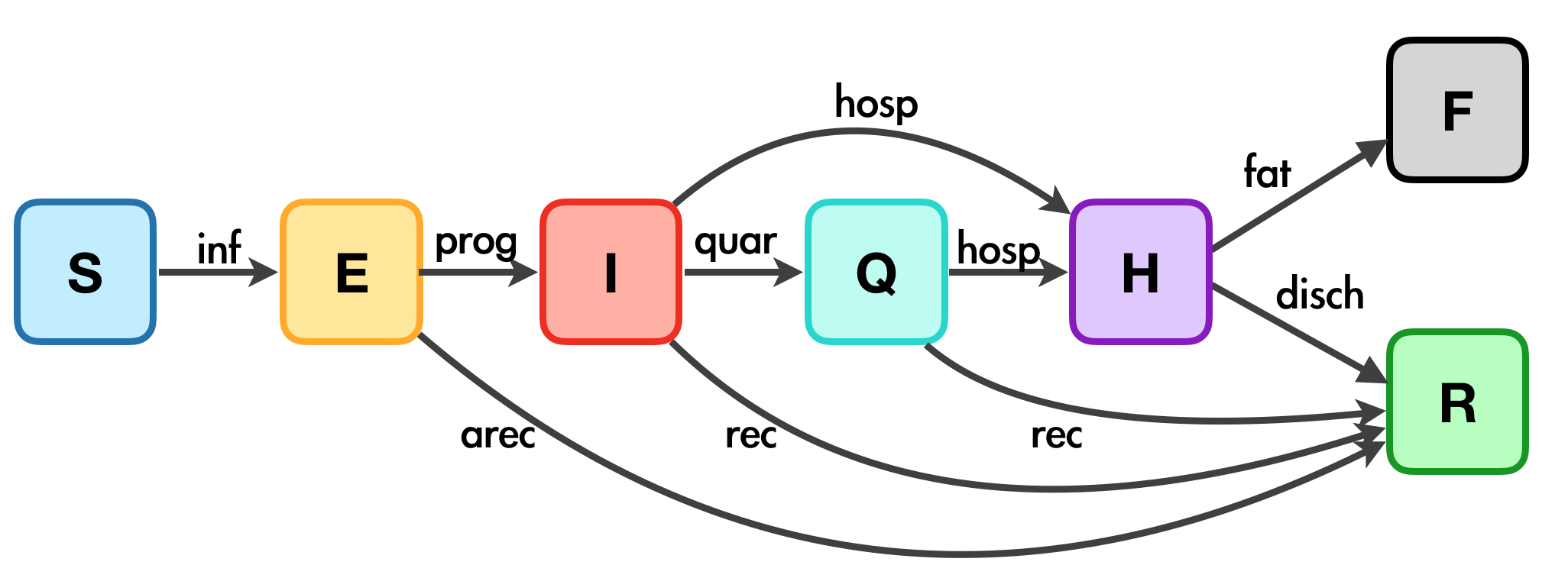
| Transitions | Description | Parameters (with default values) |
|---|---|---|
| inf | Infection due to contact with I, E and Q, which correspond to inf.i, inf.e and inf.q respectively. (See the diagram below for more details) |
act.rate.* and inf.prob.*, where * = i, e, q (See table below for more details) |
| prog | Progress from asymptomatic to symptomatic |
prog.rand = FALSE, prog.rate, prog.dist.scale = 5, prog.dist.shape = 1.5
|
| quar | From infectious to quarantine |
quar.rand = TRUE, quar.rate = 1/30
|
| hosp | From infected (both before and during quarantine) to require hospitalisation |
quar.rand = TRUE, quar.rate = 1/30
|
| rec | From infected to recovered without hospitalization |
rec.rand = FALSE, prog.dist.scale = 35, prog.dist.shape = 1.5
|
| arec | Exposed individuals recovered before symptomatic |
arec.rand = TRUE, arec.rate = 0.05
|
| disch | recovery after hospitalization |
disch.rand = TRUE, disch.rate = 1/15
|
| fat | Fatality |
fat.rate.base = 1/50, hosp.cap = 40, fat.rate.overcap = 1/25, fat.tcoeff = 0.5
|
The inf transaction results from the contact of S with at least one of I, E and Q compartments, the three sub-transactions are described in the following diagram:
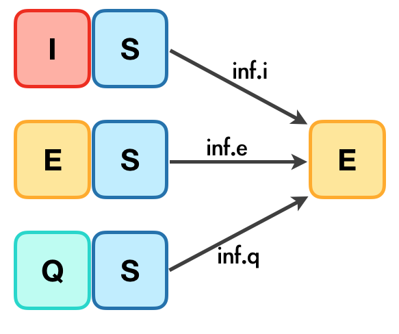
Each one of inf.i, inf.e and inf.q are controlled by two parameters:
- act.rate.* controls the number of the S that are in contact with * each day,
- inf.prob.* controls the probability that S turns into E, given that S is in contact with *,
where * is one of i, e and q respectively.
| Transitions | Description | Parameters (with default values) |
|---|---|---|
| inf.i | Infection of S due to contact with I |
act.rate.i = 10 and inf.prob.i = 0.05
|
| inf.e | Infection of S due to contact with E |
act.rate.e = 10 and inf.prob.e = 0.02
|
| inf.q | Infection of S due to contact with Q |
act.rate.q = 2.5 and inf.prob.q = 0.02
|
Simulate and inspect a baseline sirplus model
Set parameters
Here we will simulate the epidemiological data for a made-up population with 1000 susceptible individuals (S), 50 that are infected but not in the hospital or in self-quarantine (I; maybe people that are infected/symptomatic but not tested/ aware), 10 confirmed cases that have self-isolated (Q), and 1 confirmed case that has been hospitalized (H). We call this the baseline model because it uses default parameters for disease spread (i.e. no additional interventions).
library(sirplus)
s.num <- 2000  # number susceptible
i.num <- 15  # number infected
q.num <- 5  # number in self-isolation
h.num <- 1  # number in the hospital
sim_population <- s.num + i.num + q.num + h.num
nsteps <- 90 # number of steps (e.g. days) to simulate

control <- control_seiqhrf(nsteps = nsteps)
param <- param_seiqhrf()
init <- init_seiqhrf(s.num = s.num, i.num = i.num, q.num = q.num, h.num = h.num)

print(init)
## SEIQHRF Initial Conditions
## ===========================
##
## User specified control parameters:
## ---------------------------
## s.num = 2000
## i.num = 15
## q.num = 5
## h.num = 1
##
## Default control parameters:
## ---------------------------
## e.num = 0
## r.num = 0
## f.num = 0
print(control)
## SEIQHRF Control Settings
## ===========================
##
## User specified control parameters:
## ---------------------------
## nsteps = 90
##
## Default control parameters:
## ---------------------------
## nsims = 8
## prog.rand = FALSE
## quar.rand = TRUE
## hosp.rand = TRUE
## disch.rand = TRUE
## rec.rand = FALSE
## arec.rand = TRUE
## fat.rand = TRUE
## a.rand = TRUE
## d.rand = TRUE
## verbose = FALSE
## verbose.int = 0
## skip.check = FALSE
## ncores = 4
## type = SEIQHRF
## Base Modules: initialize.FUN infection.FUN recovery.FUN departures.FUN
## arrivals.FUN get_prev.FUN
print(param)
## SEIQHRF Parameters
## ===========================
##
## User specified control parameters:
## ---------------------------
##
## Default control parameters:
## ---------------------------
## inf.prob.e = 0.02
## act.rate.e = 10
## inf.prob.i = 0.05
## act.rate.i = 10
## inf.prob.q = 0.02
## act.rate.q = 2.5
## prog.rate = 0.1
## quar.rate = 0.03333333
## hosp.rate = 0.01
## disch.rate = 0.06666667
## rec.rate = 0.071
## arec.rate = 0.05
## prog.dist.scale = 5
## prog.dist.shape = 1.5
## quar.dist.scale = 1
## quar.dist.shape = 1
## hosp.dist.scale = 1
## hosp.dist.shape = 1
## disch.dist.scale = 1
## disch.dist.shape = 1
## rec.dist.scale = 35
## rec.dist.shape = 1.5
## arec.dist.scale = 35
## arec.dist.shape = 1.5
## fat.rate.base = 0.02
## hosp.cap = 40
## fat.rate.overcap = 0.04
## fat.tcoeff = 0.5
## flare.inf.point =
## flare.inf.num =
## a.rate = 2.876712e-05
## a.prop.e = 0.01
## a.prop.i = 0.001
## a.prop.q = 0.01
## ds.rate = 1.917808e-05
## de.rate = 1.917808e-05
## di.rate = 1.917808e-05
## dq.rate = 1.917808e-05
## dh.rate = 5.479452e-05
## dr.rate = 1.917808e-05
## act.rate = 1
## groups = 1
Simulate baseline
This will produce an seiqhrf object.
baseline_sim <- seiqhrf(init, control, param)
baseline_sim
## SEIQHRF Model Simulation
## =======================
## Model class: seiqhrf
##
## Simulation Summary
## -----------------------
## Model type: SEIQHRF
## Number of simulations: 8
## Number of time steps: 90
##
## Model Output (variable names)
## -----------------------
## s.num i.num num se.flow is.flow iq.flow iq2h.flow hf.flow
## ds.flow de.flow di.flow dq.flow dh.flow dr.flow a.flow
## a.e.flow a.i.flow a.q.flow e.num r.num q.num h.num f.num
Extract summary of the simulation
summary(baseline_sim)
## Peaks of SEIQHRF Model Simulation:
## ===============================
##           Max Time
## s.num 2000.00    1
## e.num  329.38   20
## i.num  520.00   26
## q.num  115.25   29
## h.num   60.75   36
## r.num 1926.75   90
## f.num    3.12   42
ls.str(summary(baseline_sim))
## e.num : List of 4
##  $ mean : Named num [1:90] NaN 7.25 16.12 27.12 34.25 ...
##  $ sd   : Named num [1:90] NA 2.82 6.36 6.58 10.71 ...
##  $ CI   : num [1:90, 1:2] NaN 1.73 3.67 14.23 13.25 ...
##  $ qntCI: num [1:90, 1:2] NA 4.17 7.53 14.62 16.45 ...
## f.num : List of 4
##  $ mean : Named num [1:90] NaN 0 0 0 0 0 0 0 0.25 0.25 ...
##  $ sd   : Named num [1:90] NA 0 0 0 0 ...
##  $ CI   : num [1:90, 1:2] NaN 0 0 0 0 ...
##  $ qntCI: num [1:90, 1:2] NA 0 0 0 0 0 0 0 0 0 ...
## h.num : List of 4
##  $ mean : Named num [1:90] NaN 1.12 1.12 1.25 1.38 ...
##  $ sd   : Named num [1:90] NA 0.641 0.641 0.463 0.744 ...
##  $ CI   : num [1:90, 1:2] NaN -0.1311 -0.1311 0.3427 -0.0833 ...
##  $ qntCI: num [1:90, 1:2] NA 0.175 0.175 1 1 ...
## i.num : List of 4
##  $ mean : Named num [1:90] 15 14.2 14.2 15.5 19.8 ...
##  $ sd   : Named num [1:90] 0 1.16 1.67 2.27 3.41 ...
##  $ CI   : num [1:90, 1:2] 15 12 11 11.1 13.1 ...
##  $ qntCI: num [1:90, 1:2] 15 12.2 11.3 12.3 13.7 ...
## q.num : List of 4
##  $ mean : Named num [1:90] NaN 5.5 6.25 7.25 7.75 ...
##  $ sd   : Named num [1:90] NA 1.07 1.49 2.05 2.43 ...
##  $ CI   : num [1:90, 1:2] NaN 3.4 3.33 3.23 2.98 ...
##  $ qntCI: num [1:90, 1:2] NA 4.17 4.17 4.17 4.17 ...
## r.num : List of 4
##  $ mean : Named num [1:90] NaN 0.25 0.875 2.25 4.125 ...
##  $ sd   : Named num [1:90] NA 0.463 0.991 2.765 3.044 ...
##  $ CI   : num [1:90, 1:2] NaN -0.657 -1.067 -3.169 -1.842 ...
##  $ qntCI: num [1:90, 1:2] NA 0 0 0 0.35 ...
## s.num : List of 4
##  $ mean : Named num [1:90] 2000 1993 1982 1967 1954 ...
##  $ sd   : Named num [1:90] 0 2.88 6.86 9.09 13.45 ...
##  $ CI   : num [1:90, 1:2] 2000 1987 1969 1950 1927 ...
##  $ qntCI: num [1:90, 1:2] 2000 1988 1974 1957 1937 ...
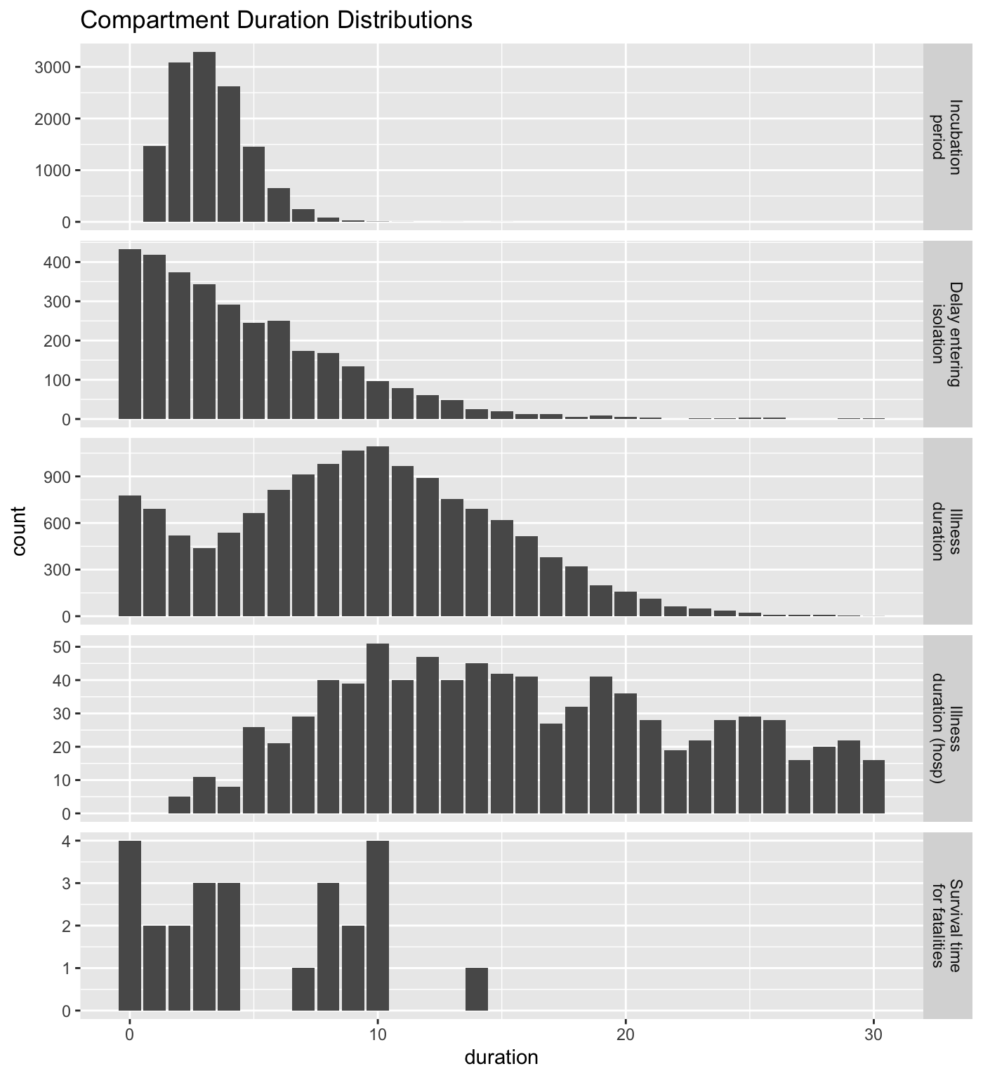
Inspect baseline transition distributions
The sirplus model controls transitions between compartments, i.e. a change in state for an individual (e.g. going from self-isolation to hospital), using a variety of transition parameters. You can use the plot() functions, and set parameter method as times to examine the distributions of timings for various transitions based on these parameters. In the case of a disease with observed data available, these plots can be used to sanity check parameter settings.
plot(baseline_sim, "times")
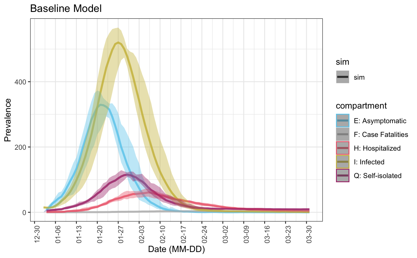
Plot baseline sirplus results
To visualise your sirplus model, you can plot the change in prevalence (i.e. people) over time in each compartment. By default, this plotting function shows the mean count across all simulations and the 95th quantile in the ribbon. You can hide the CI by setting parameter ci to FALSE.
plot(baseline_sim,
     start_date = lubridate::ymd("2020-01-01"),
     comp_remove = c('s.num', 'r.num'),
     plot_title = 'Baseline Model')
## Scale for 'colour' is already present. Adding another scale for 'colour',
## which will replace the existing scale.
## Warning: Removed 4 row(s) containing missing values (geom_path).
Run an experiment
With the sirplus package you can also set up experiments. We will set up two experiments here:
- Experiment #1: One week after the beginning of the epidemic, schools and non-essential businesses are closed to encourage social distancing. This causes the act.rate to gradually drop from 10 to 6 over the course of the next week. In this experiment, we imagine these policies are never lifted, so act.rate remains at 6 for the duration of the simulation.
- Experiment #2: Again, one week after the beginning of the epidemic, social distancing policies are put into place resulting in act.rate dropping from 10 to 6 over the next week. But after two weeks these policies are lifted and the act.rate returns to normal within the next week.
# Experiment #1
vals <- c(10, 7)
timing <- c(7, 14)
act_rate <- vary_param(nstep = nsteps, vals = vals, timing = timing)

control <- control_seiqhrf(nsteps = nsteps)
param <- param_seiqhrf(act.rate.e = act_rate, act.rate.i = act_rate * 0.5)
init <- init_seiqhrf(s.num = s.num, i.num = i.num, q.num = q.num, h.num = h.num)
sim_exp <- seiqhrf(init, control, param)

# Experiment #2
vals <- c(10, 7, 7, 10)
timing <- c(7, 14, 21, 28)
act_rate_relax <- vary_param(nstep = nsteps, vals = vals, timing = timing)

param <- param_seiqhrf(act.rate.e = act_rate_relax, act.rate.i = act_rate_relax * 0.5)
sim_exp_relax <- seiqhrf(init, control, param)

# Compare experiments 1 and 2 to the baseline simulation
plot(list("Baseline" = baseline_sim, "Closures" = sim_exp,
          "Closures (2 mo)" = sim_exp_relax),
     start_date = lubridate::ymd("2020-01-01"),
     comp_remove = c('s.num', 'r.num'), plot_title = 'Closures Experiment')
## Scale for 'colour' is already present. Adding another scale for 'colour',
## which will replace the existing scale.
## Warning: Removed 64 row(s) containing missing values (geom_path).
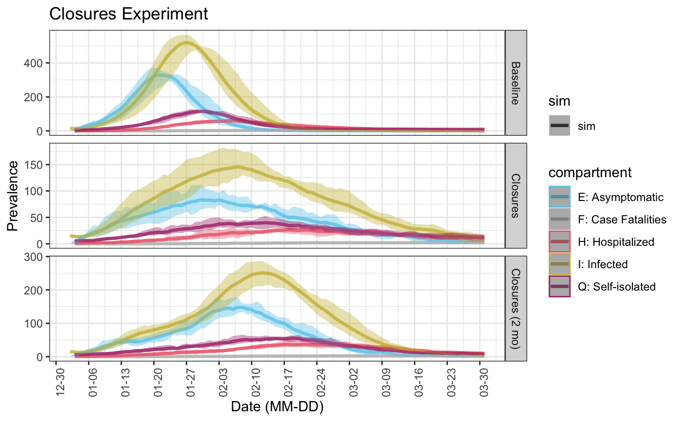
From these results we see that this policy would likely reduce the peak number of infections from 500 to 300 and would “flatten the curve” for infections and thus hospitalizations (the peak in number of infected people is lower, but the number of people infected declines more slowly after the peak of the epidemic than in the baseline model).
Visualize sirplus: Advanced Plotting Options
A. Adding known data
You can use the plot() function to include known compartment values alongside your simulations by supplying the known values as a dataframe to parameter known. This can be helpful when wanting to know how well experiments are simulating the epidemic progression to the point where you have data.
For example, if we know the hospitalization numbers have been growing exponentially (by 0.2) at each step, we can see how that compares to our experiments.
known <- data.frame('time' = seq(1:30), 'h.num' =  seq(0, 10, by=0.2)[1:30])

plot(list("Baseline" = baseline_sim, "Closures" = sim_exp,
          "Closures (2 mo)" = sim_exp_relax), time_lim = 45,
     known = known,
     start_date = lubridate::ymd("2020-01-01"),
     comp_remove = c('s.num', 'r.num', 'e.num', 'i.num', 'q.num'),
     plot_title = 'Closures Experiment')
## Scale for 'colour' is already present. Adding another scale for 'colour',
## which will replace the existing scale.
## Warning: Removed 32 row(s) containing missing values (geom_path).
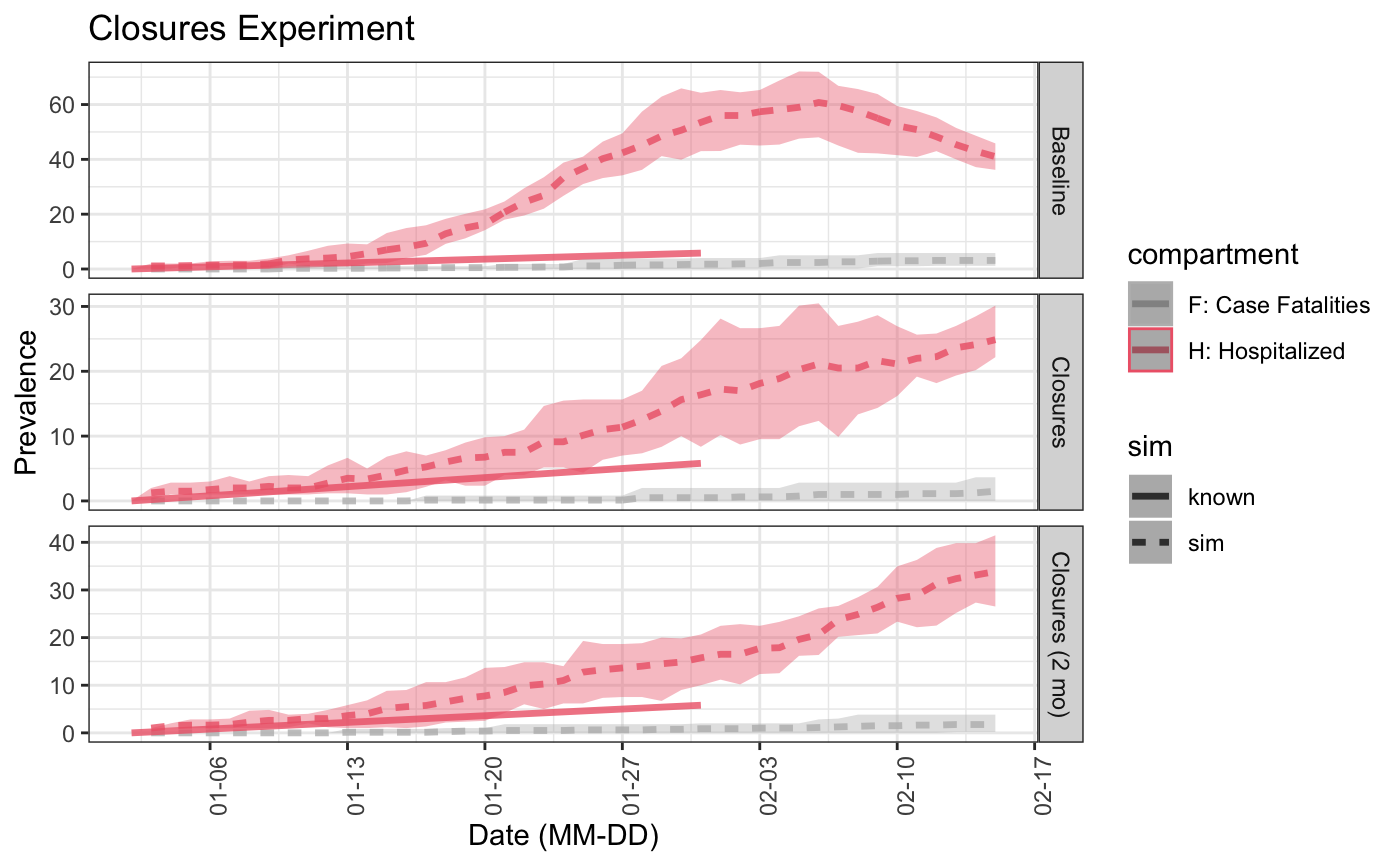 From this, we can see that the closure for 2 months is slightly pessimistic, while the closures simulation is close to the known hospitalization rate.
B. Plotting compartment separately
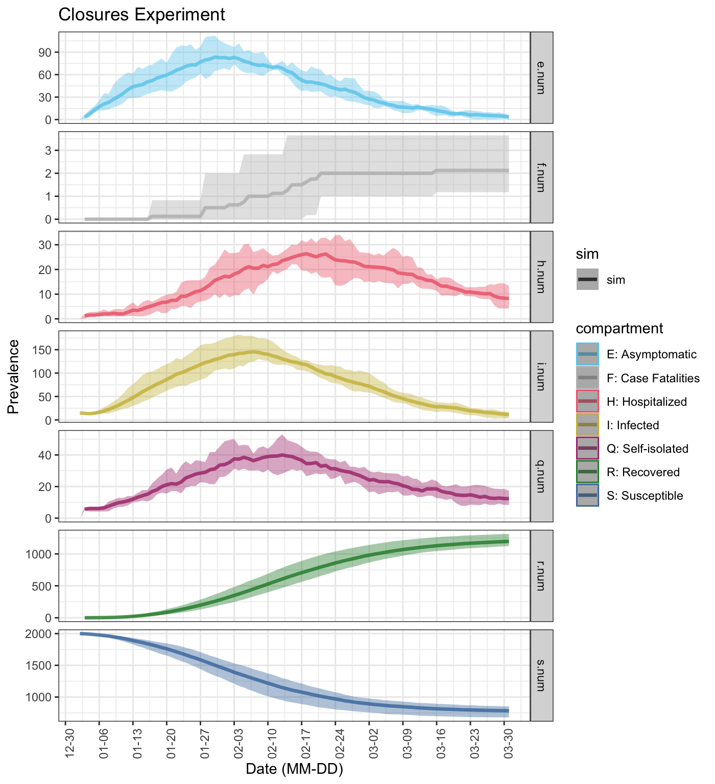
You can use the plot() function to plot counts for each compartment separately by specifying sep_compartments as ‘y’. This can be useful when visualizing compartments on different scales (e.g. i.num v f.num) without using log transformations.
plot(sim_exp,
     sep_compartments = TRUE,
     start_date = lubridate::ymd("2020-01-01"),
     plot_title = 'Closures Experiment')
## Scale for 'colour' is already present. Adding another scale for 'colour',
## which will replace the existing scale.
## Warning: Removed 5 row(s) containing missing values (geom_path).
C. Weekly hospitalization numbers
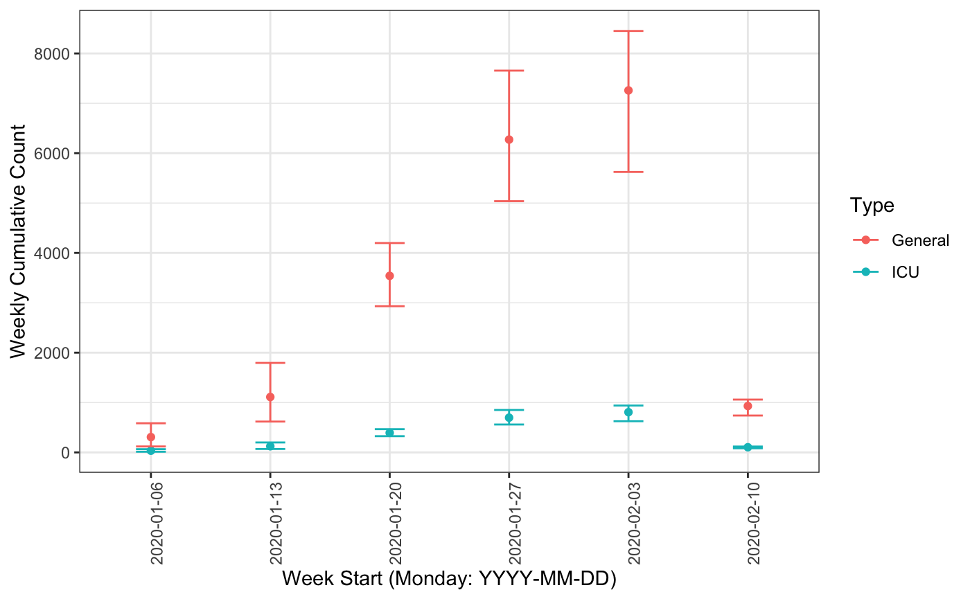
Use the plot() function with parameter method = "weekly_local" to extract and plot the number of weekly expected patients in a hospital. If return_df is TRUE, the function returns a dataframe that generates the plot, otherwise, it returns a ggplot object.
This function takes the following input:
-
sims: Single or list of outputs from simulate.seiqhrf(). -
market.share: Percent of cases in your model population (s.num) that are anticipated at the hospital of interest. Default = 4% (0.04). -
icu_percent: Percent of hospitalised cases are are likely to need treatment in an intensive care unit (ICU). Default = 10% (0.1). -
start_date: Epidemic start date. Default isNA. -
show_start_date: First date to show in plots. Default is to show from beginning -
time_lim: Number of days (nsteps) to include. Default = 90. -
total_population: True population size. This parameter is only needed if the simulation size (s.num) was smaller than the true population size (i.e. scaled down) to reduce computational cost. -
sim_population: Size of simulation population. Only needed if providingtotal_population.
library(lubridate)
plot(baseline_sim, method = "weekly_local",
     time_lim = 40,
     start_date = ymd("2020-01-01"),
     show_start_date = ymd("2020-01-06"),
     total_population = 40000,
     sim_population = sim_population,
     return_df = TRUE)
## Scalling w.r.t total population  h.num   ci5  ci95
## 1 1.375 1.000 2.825
## 2 1.500 1.000 3.000
## 3 1.500 0.175 3.000
## 4 1.875 0.175 3.825
## 5 3.250 2.000 5.000
## 6 3.750 1.175 6.650
## $plot
##
## $result
## # A tibble: 6 x 7
##   yr_wk      h.num h.ci5 h.ci95 icu.num icu.ci5 icu.ci95
##   <fct>      <dbl> <dbl>  <dbl>   <dbl>   <dbl>    <dbl>
## 1 2020-01-06  307.  119.   584.    34.1    13.3     64.9
## 2 2020-01-13 1111.  618.  1795.   123.     68.7    199.
## 3 2020-01-20 3540. 2932.  4198.   393.    326.     466.
## 4 2020-01-27 6272. 5038.  7656.   697.    560.     851.
## 5 2020-02-03 7259. 5624.  8450.   807.    625.     939.
## 6 2020-02-10  931.  740.  1059.   103.     82.2    118.
References
Churches, Timothy, and Louisa Jorm. 2020. “COVOID: A flexible, freely available stochastic individual contact model for exploring COVID-19 intervention and control strategies.” JMIR Preprints. https://doi.org/10.2196/preprints.18965.
Jenness, Samuel M, Steven M Goodreau, and Martina Morris. 2018. “EpiModel: An R Package for Mathematical Modeling of Infectious Disease over Networks.” Journal of Statistical Software 84 (April). https://doi.org/10.18637/jss.v084.i08.