Using stochastic parameters
Last updated: 25 April 2020
stochastic_parameters.Rmdlibrary(sirplus) library(ggplot2) s.num <- 1000 # number susceptible i.num <- 15 # number infected q.num <- 5 # number in self-isolation h.num <- 1 # number in the hospital nsteps <- 101 # number of steps (e.g. days) to simulate nsims <- 20 control <- control_seiqhrf(nsteps = nsteps, nsims = nsims) init <- init_seiqhrf(s.num = s.num, i.num = i.num, q.num = q.num, h.num = h.num)
Instead of running all nsims simulations with fixed parameter values, sirplus enables the act.rate.* and inf.prob.* (where * is one of i, e and q) to be randomly generated from a probability distribution, which can be seen as a prior.
1. Using fixed parameter values across time with default prior distributions
We use function select_prior to specify priors. If default prior distributions are desired, we only need to input a vector of the names of parameter that are to be generated stochastically.
If not specified, the default values are as follows:
| Variables | Distribution | Parameters (of the prior distribution) and default values |
|---|---|---|
| act.rate.* | Gaussian |
mean = param$act.rate.* and sd = 0.1
|
| inf.prob.* | Beta |
a = 50 and b is calculated s.t. the expectation equals param$inf.prob.*
|
param0 <- param_seiqhrf()
priors0 <- select_prior(param0, c("act.rate.q", "act.rate.i", "inf.prob.i", "inf.prob.e"))
priors0
## Prior distributions for SEIQHRF Parameters
## ===========================================
## act.rate.q : N( mean = 2.5 , sd = 0.1 )
## act.rate.i : N( mean = 10 , sd = 0.1 )
## inf.prob.i : Beta( a = 50 , b = 950 ), mean = 0.05 , s.e = 0.007
## inf.prob.e : Beta( a = 50 , b = 2450 ), mean = 0.02 , s.e = 0.003
## ===========================================
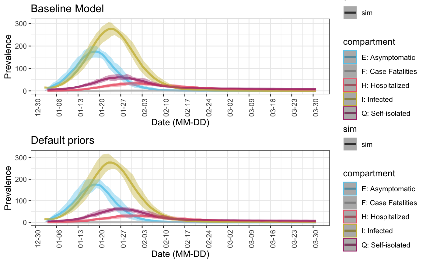
We can see how the simulation is different from the baseline simulation which uses constant parameters.
baseline_sim <- seiqhrf(init, control, param0)
baseline_plot <- plot(baseline_sim, start_date = lubridate::ymd("2020-01-01"), comp_remove = c('s.num', 'r.num'), plot_title = 'Baseline Model')

sim0 <- seiqhrf(init, control, param0, priors0)
sim0_plot <- plot(sim0, start_date = lubridate::ymd("2020-01-01"), comp_remove = c('s.num', 'r.num'), plot_title = 'Default priors')

gridExtra::grid.arrange(baseline_plot, sim0_plot)
2. Using time varying prior distributions with default prior distributions
If a parameter in param is a vector (i.e. its value varies over time), its prior distribution will be different across time points as well.
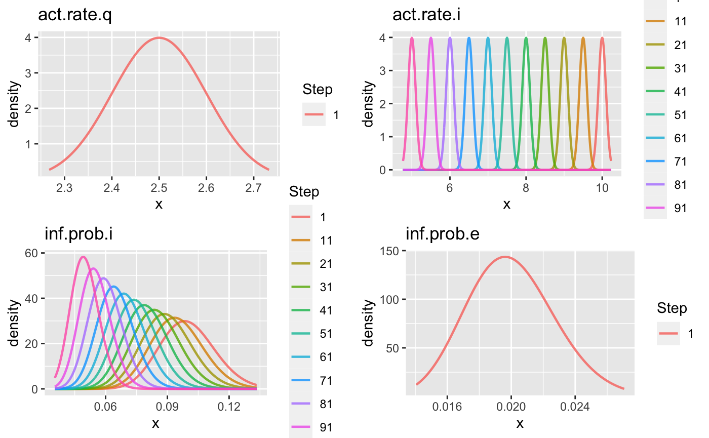
param1 <- param_seiqhrf(act.rate.i = seq(10, 5, -0.05), inf.prob.i = seq(0.1, 0.05, -0.0005))
priors1 <- select_prior(param1, c("act.rate.q", "act.rate.i", "inf.prob.i", "inf.prob.e"))
priors1
## Prior distributions for SEIQHRF Parameters
## ===========================================
## act.rate.q : N( mean = 2.5 , sd = 0.1 )
## act.rate.i : N( mean = 10, 9.95, 9.9, ... , sd = 0.1, 0.1, 0.1, ... )
## inf.prob.i : Beta( a = 50, 50, 50, ... , b = 450, 452.513, 455.051, ... ), mean = 0.1, 0.1, 0.099, ... , s.e = 0.013, 0.013, 0.013, ...
## inf.prob.e : Beta( a = 50 , b = 2450 ), mean = 0.02 , s.e = 0.003
## ===========================================
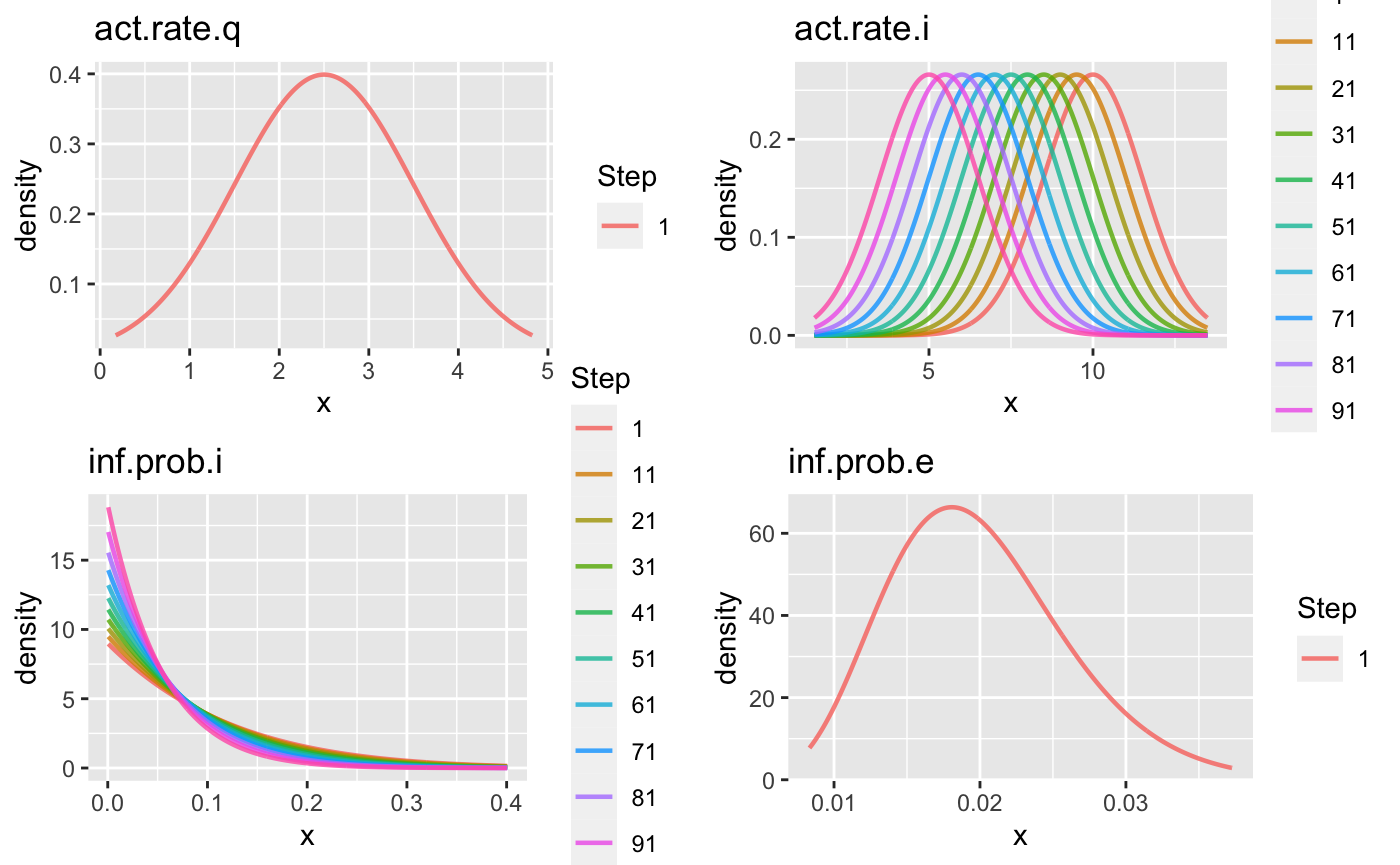
We can plot the priors and see how they change with time. If nstep is larger than 10, the prior curves of only 10 (evenly distributed) time points will be plotted (see the Step label).
gg1 <- plot(priors1)
gridExtra::grid.arrange(gg1[[1]], gg1[[2]], gg1[[3]], gg1[[4]])
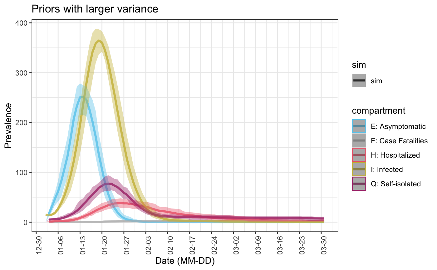
sim1 <- seiqhrf(init, control, param1, priors1)
plot(sim1, start_date = lubridate::ymd("2020-01-01"), comp_remove = c('s.num', 'r.num'), plot_title = 'Priors with larger variance')
3. Using time varying parameter values with the same prior distribution
Another alternative to incorporate time varying parameters, is to simulate only for the first time point, parameters used for the latter time points are shifted from the input values in param by the same amount as the first time point. By doing so, we preserve the desired trend/change of the parameter across time by avoiding excessive variance, while allowing some randomness in the intercept. This can by achieved by simply setting shift_only == TRUE.
priors2 <- select_prior(param1, c("act.rate.q", "act.rate.i", "inf.prob.i", "inf.prob.e"), shift_only = TRUE)
sim2 <- seiqhrf(init, control, param1, priors2)
Take act.rate.i for example, the increment between time points are preserved, but for each simulation the starting point is randomly generated.
## Generated act.rate.i:
##      t = 1 t = 2 t = 3
## sim1 10.08 10.03  9.98
## sim2  9.86  9.81  9.76
## sim3 10.10 10.05 10.00
##
##
## Original input of act.rate.i in param:
## t = 1 t = 2 t = 3
## 10.00  9.95  9.90
4. Using user specified prior distributions
We can also manually specify the parameters in the prior distributions. For example, the following parameter setting results in distributions with larger variance.
priors3 <- select_prior(param1, c("act.rate.q", "act.rate.i", "inf.prob.i", "inf.prob.e"), prior.dist = c("gaussian", "gaussian", "beta", "beta"),
                       prior.pars = list(list(sd = 1), list(sd = 1.5), list(a = 1), list(a = 10)))
priors3
## Prior distributions for SEIQHRF Parameters
## ===========================================
## act.rate.q : N( mean = 2.5 , sd = 1 )
## act.rate.i : N( mean = 10, 9.95, 9.9, ... , sd = 1.5, 1.5, 1.5, ... )
## inf.prob.i : Beta( a = 1, 1, 1, ... , b = 9, 9.05, 9.101, ... ), mean = 0.1, 0.1, 0.099, ... , s.e = 0.09, 0.09, 0.09, ...
## inf.prob.e : Beta( a = 10 , b = 490 ), mean = 0.02 , s.e = 0.006
## ===========================================
gg3 <- plot(priors3)
gridExtra::grid.arrange(gg3[[1]], gg3[[2]], gg3[[3]], gg3[[4]])
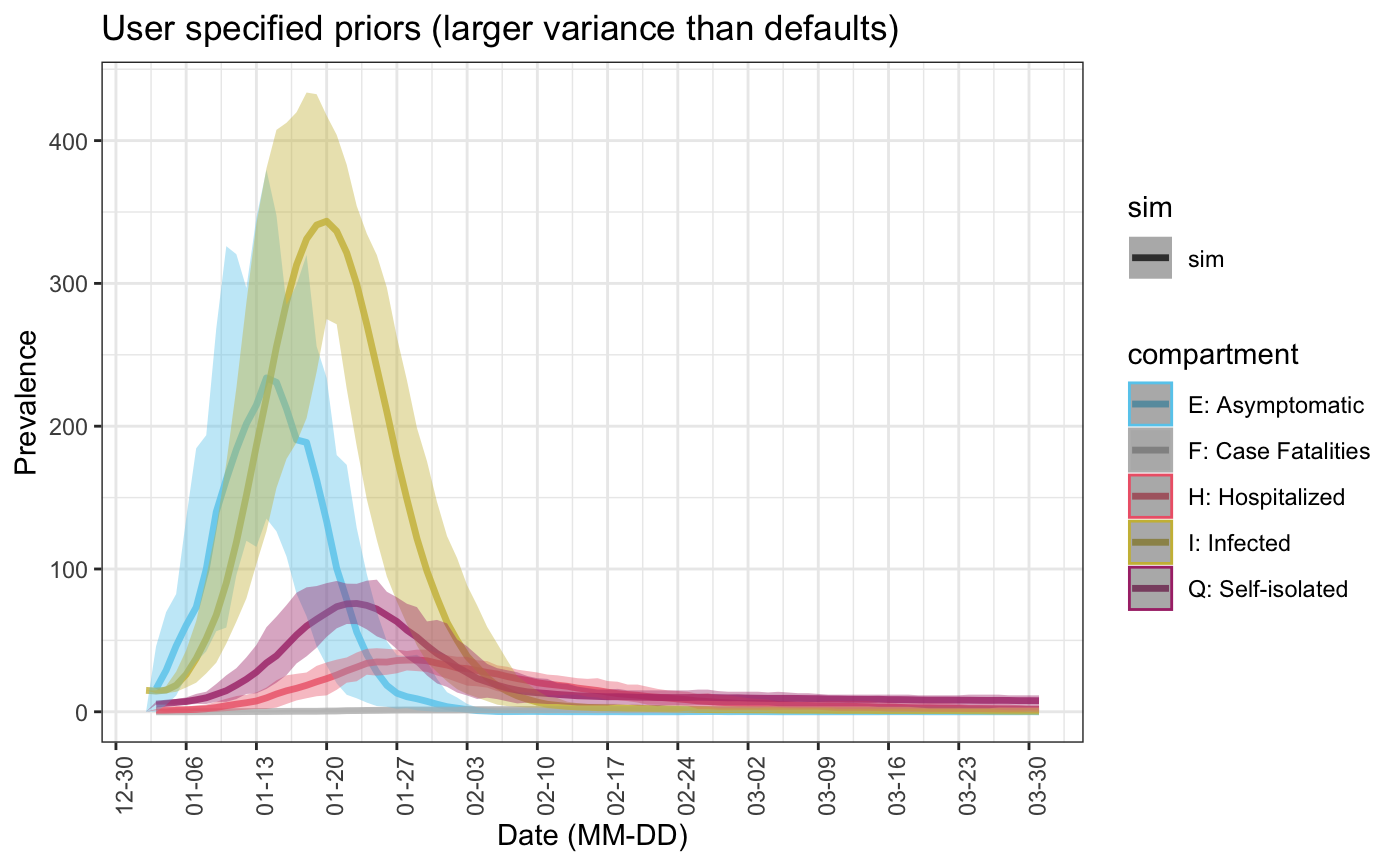
As expected, this leads to a larger variance in simulations as well:
sim3 <- seiqhrf(init, control, param1, priors3)
plot(sim3, start_date = lubridate::ymd("2020-01-01"), comp_remove = c('s.num', 'r.num'), plot_title = 'User specified priors (larger variance than defaults)')
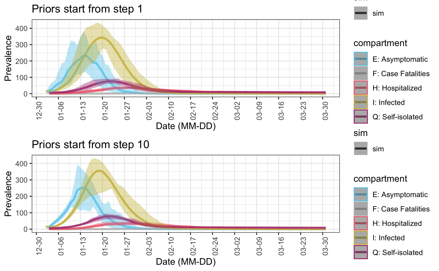
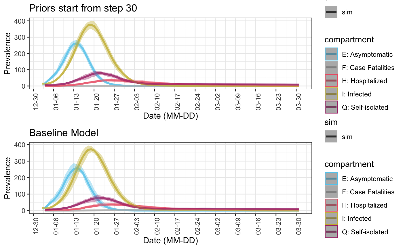
5. Specifying starting point of stochastic model parameters
In the examples above, all models parameters are generated from given or default prior distributions from the first time point. But it is also possible to use fixed parameters values at the first several time points, since it is generally true that the more recent predictions should have smaller variances. In this case, we can specify the starting points of applying random model parameters through starting.point in function select_prior. This can either be a number (i.e. the same starting point is applied to all parameters with priors), or a vector of the same length as pars.
priors4 <- select_prior(param1, c("act.rate.q", "act.rate.i", "inf.prob.i", "inf.prob.e"), prior.dist = c("gaussian", "gaussian", "beta", "beta"),
                        prior.pars = list(list(sd = 1), list(sd = 1.5), list(a = 1), list(a = 10)), starting.point = 10)
priors4
## Prior distributions for SEIQHRF Parameters
## ===========================================
## act.rate.q : N( mean = 2.5 , sd = 1 ), starting at step  10
## act.rate.i : N( mean = 10, 9.95, 9.9, ... , sd = 1.5, 1.5, 1.5, ... ), starting at step  10
## inf.prob.i : Beta( a = 1, 1, 1, ... , b = 9, 9.05, 9.101, ... ), mean = 0.1, 0.1, 0.099, ... , s.e = 0.09, 0.09, 0.09, ..., starting at step 10
## inf.prob.e : Beta( a = 10 , b = 490 ), mean = 0.02 , s.e = 0.006, starting at step 10
## ===========================================
Finally, put together simulations where priors are applied at different time points, we can see as expected that the later random parameters start, the smaller the variance become and the closer it is to the baseline simulation where parameters are always constants.