10 Clustering and cell annotation
10.1 Clustering Methods
Once we have normalized the data and removed confounders we can carry out analyses that are relevant to the biological questions at hand. The exact nature of the analysis depends on the dataset. Nevertheless, there are a few aspects that are useful in a wide range of contexts and we will be discussing some of them in the next few chapters. We will start with the clustering of scRNA-seq data.
10.1.1 Introduction
One of the most promising applications of scRNA-seq is de novo discovery and annotation of cell-types based on transcription profiles. Computationally, this is a hard problem as it amounts to unsupervised clustering. That is, we need to identify groups of cells based on the similarities of the transcriptomes without any prior knowledge of the labels. Moreover, in most situations we do not even know the number of clusters a priori. The problem is made even more challenging due to the high level of noise (both technical and biological) and the large number of dimensions (i.e. genes).
When working with large datasets, it can often be beneficial to apply some sort of dimensionality reduction method. By projecting the data onto a lower-dimensional sub-space, one is often able to significantly reduce the amount of noise. An additional benefit is that it is typically much easier to visualize the data in a 2 or 3-dimensional subspace. We have already discussed PCA (chapter 6.6.2) and t-SNE (chapter 6.6.2).
Challenges in clustering
- What is the number of clusters k?
- What defines a good clustering?
- What is a cell type?
- Scalability: in the last few years the number of cells in scRNA-seq experiments has grown by several orders of magnitude from ~\(10^2\) to ~\(10^6\)
10.1.2 Unsupervised clustering methods
Three main ingredients of a complete clustering method:
Measure of similarity: how do we quantify how close two data points are?
Quality function: how do we decide how “good” is a clustering/partition?
Algorithm: how to find the clustering whose quality function is optimized?
10.1.2.1 Hierarchical clustering
Hierarchical clustering is basically the only type of clustering algorithm that does not seek to optimize a quality function, because it builds a hierarchy of clusters, instead of one single clustering result as the output.
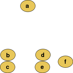
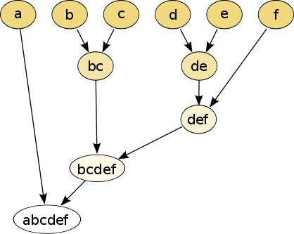
There are two types of strategies:
- Agglomerative (bottom-up): each observation starts in its own cluster, and pairs of clusters are merged as one moves up the hierarchy.
- Divisive (top-down): all observations start in one cluster, and splits are performed recursively as one moves down the hierarchy.
10.1.2.2 k-means clustering
Measure of similarity: Euclidean distance
Quality function: Within cluster distance
Algorithm:
Advantage: Fast
Drawbacks:
- Sensitive to initial clustering
- Sensitive to outliers
- Need to specify K
- Tend to find clusters of similar sizes
Tools related to K-means: SC3
10.1.2.3 Graph-based methods
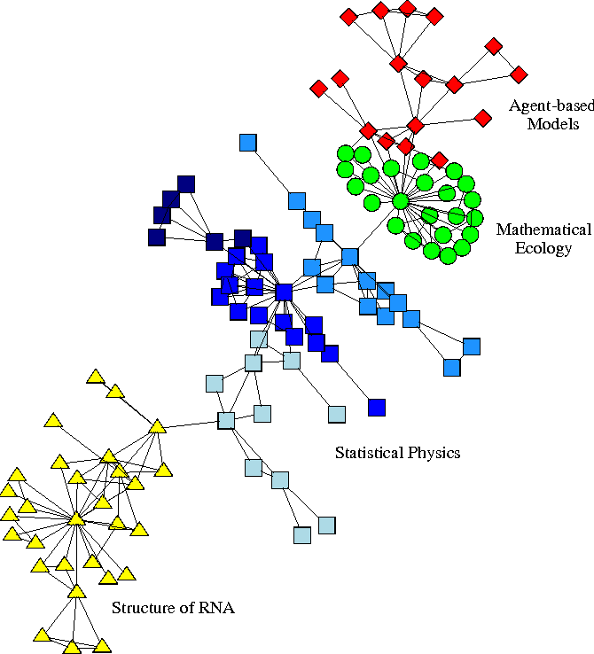
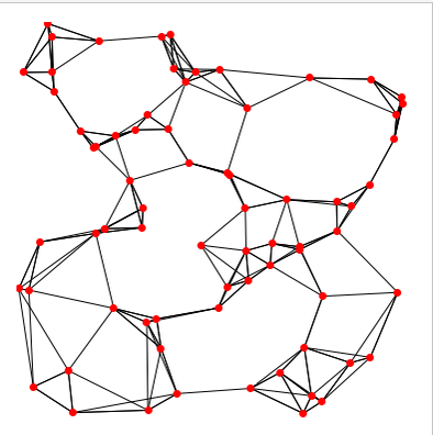
Real world networks usualy display big inhomogeneities or community structure. Communities or clusters or modules are groups of vertices which probably share common properties and/or play similar roles whithin the graph. In recent years there has been a lot of interest in detecting communities in networks in various domains.
Some of these community detection methods can be applied
to scRNA-seq data by building a graph where each vertice represents a cell
and (weight of) the edge measures similarity between two cells.
Actually, graph-based clustering is the most popular clustering algorithm in
scRNA-seq data analysis, and has been reported to have outperformed other
clustering methods in many situations (Freytag et al. 2018).
10.1.2.3.1 Why do we want to represent the data as a graph?
- Memory effectiveness: A (complete) graph can be thought as an alternative expression of similarity matrix. Current methods (discuss later) aim to build sparse graphs, which ease the memory burden.
- Curse of dimensionality: All data become sparse in high-dimensional space and therefore similarities measured by Euclidean distances etc are generally low between all objects.
10.1.2.3.2 Building a graph
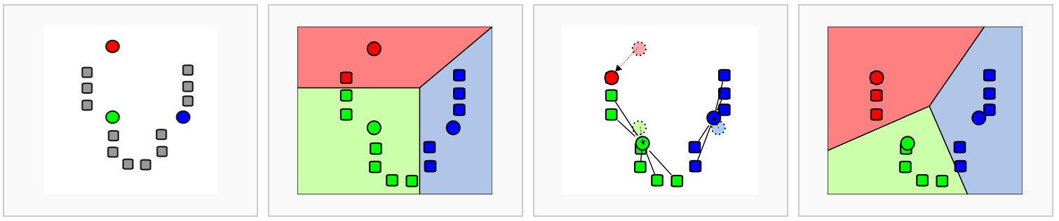
- Step1: Build an unweighted K-nearest neighbour (KNN) graph
- Step2: Add weights, and obtain a shared nearest neighbour (SNN) graph
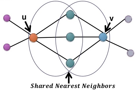
There are two ways of adding weights: number and rank.
- number: The number of shared nodes between \(u\) and \(v\), in this case, 3.
- rank: A measurement of the closeness to their common nearest neighbours. ((???))
Details of rank :
Main idea: The closeness of two people is defined by their closest common friend.
For each node, say \(u\), we can rank its 5 neighbours according to their closeness to \(u\), and we can do the same with \(v\).
Denote the three shared neighbours as \(x_1\), \(x_2\) and \(x_3\), so rank(\(x_1, u\)) = 1 means \(x_1\) is the closest neighbour of \(u\).
The idea is, if \(x_1\) is also the closest to \(v\), then \(u\) and \(v\) should have a larger similarity, or weight.
So we summarize the overall closeness of \(x_1\) with both \(u\) and \(v\) by taking an average: \(\dfrac{1}{2}(\text{rank}(x_1, u), \text{rank}(x_1, v))\).
Then we find the one with the largest closeness, \(s(u, v) = \min \left[ \dfrac{1}{2}(\text{rank}(x_i, u), \text{rank}(x_i, v)) \vert i = 1, 2, 3\right]\).
The final expression of weight:
\[ w(u, v) = K - s(u, v).\]
10.1.2.3.3 Quality function (Modularity)
Modularity (Newman and Girvan 2004) is not the only quality function for graph-based clustering,
but it is one of the first attempts to embed in a compact form many questions including
the definition of quality function and null model etc.
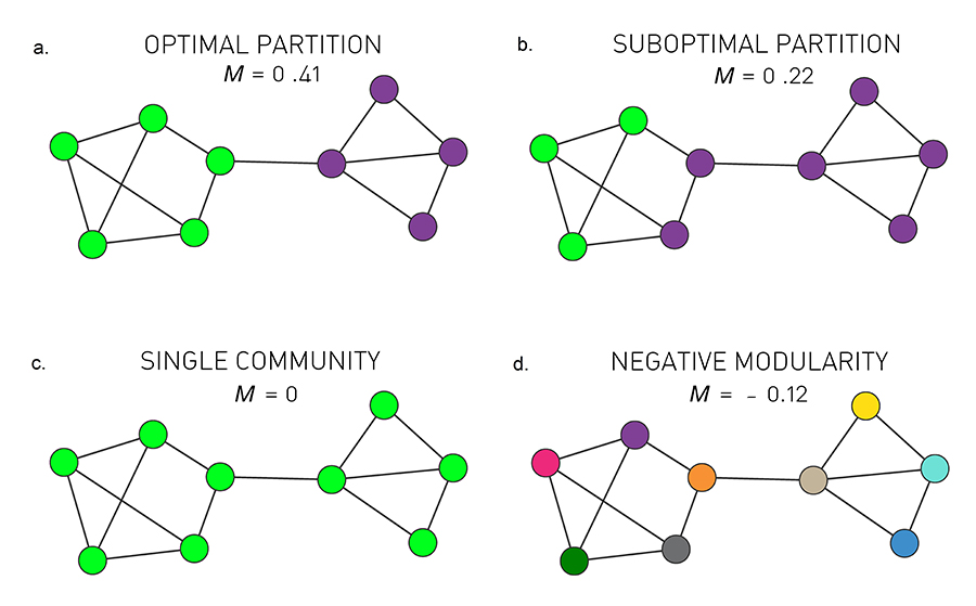
The idea of modularity: A random graph should not have a cluster structure.
The more “quality” a partition has compared to a random graph, the “better” the partition is.
Specifically, it is defined by:
the quality of a partition on the actual graph \(-\) the quality of the same partition on a random graph
quality : Sum of the weights within clusters
random graph : a copy of the original graph, with some of its properties, but without community structure. The random graph defined by modularity is: each node has the same degree as the original graph.
\[ Q \propto \sum_{i, j} A_{i, j} \delta(i, j) - \sum_{i, j} \dfrac{k_i k_j}{2m} \delta(i, j)\]
\(A_{i, j}\): weight between node \(i\) and \(j\);
\(\delta(i, j)\): indicator of whether \(i\) and \(j\) are in the same cluster;
\(k_i\): the degree of node \(i\) (the sum of weights of all edges connected to \(i\));
\(m\): the total weight in the all graph.
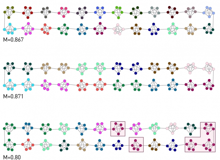
1. Resolution limit.
Short version: Modularity maximization forces small communities into larger ones.
Longer version: For two clusters \(A\) and \(B\), if \(k_A k_B < 2m\) then modularity increases by merging A and B into a single cluster, even if A and B are distinct clusters.
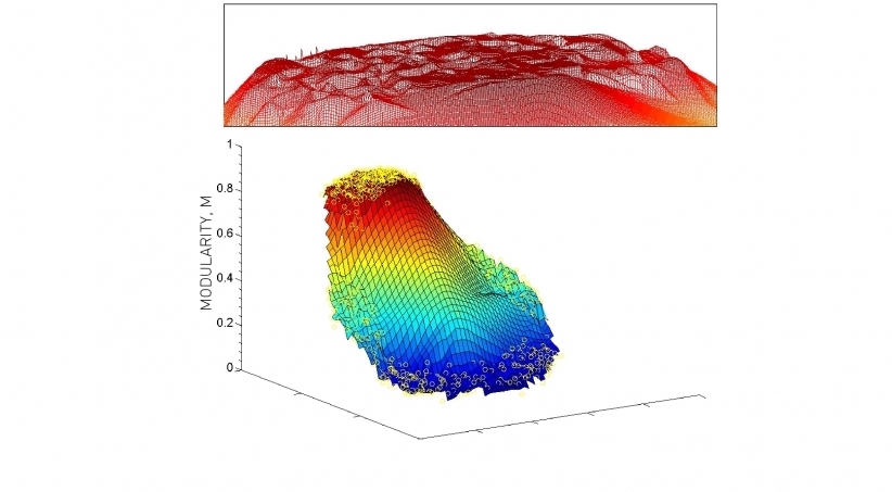
2. Bad, even random partitions may have a high modularity.
- Networks lack a clear modularity maxima.
10.1.2.3.4 Algorithms :
Modularity-based clustering methods implemented in single cell analysis are mostly greedy algorithms, that are very fast, although not the most accurate approaches.
Louvain: (Blondel et al. 2008)
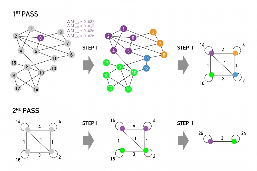
Leiden:(Traag, Waltman, and Eck 2019)
Improved Louvain, hybrid of greedy algorithm and sampling technique
10.1.2.3.5 Advantages:
-Fast
-No need to specify \(k\)
10.1.2.4 Consensus clustering (more robustness, less computational speed)
10.1.2.4.1 Motivation (Two problems of \(K\)-means):
- Problem1: sensitive to initial partitions
Solution: Run multiple iterations of \(K\)-means on different subsamples of the original dataset, with different initail partitions.
- Problem2: the selection of \(K\).
Solution: Run \(K\)-means with a range of \(K\)’s.
10.1.2.4.2 Algorithm of consensus clustering (simpliest version):
for(k in the range of K){
for(each subsample of the data){
for(iteration in 1:1000){
kmeans(subsample, k) # each iteration means a different initial partition
save partition
}
}
return consensus clustering result of k
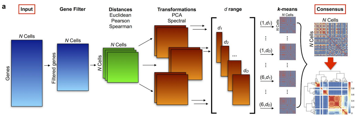
}10.1.2.4.3 Subsample obtained by dimensional reduction:
steps of PCA:
i) tranformation of the similarity matrix.
ii) ranking eigen vectors according to their accoring eigen values in decreasing order.
iii) need to decide how many (\(d\)) PC’s or eigenvalues we wants to reduce to.
In SC3,
i) considers two types of transformation:
the one with traditional PCA and the associated graph Laplacian.
iii) User may specify a range of \(d\), or use the default range suggested by the authors according to their experience with empirical results.
10.1.2.4.4 Consensus clustering (combining multiple clustering results):
- Step1: Represent each partition as a matrix:
Say we partitioned four data points into 2 clusters.
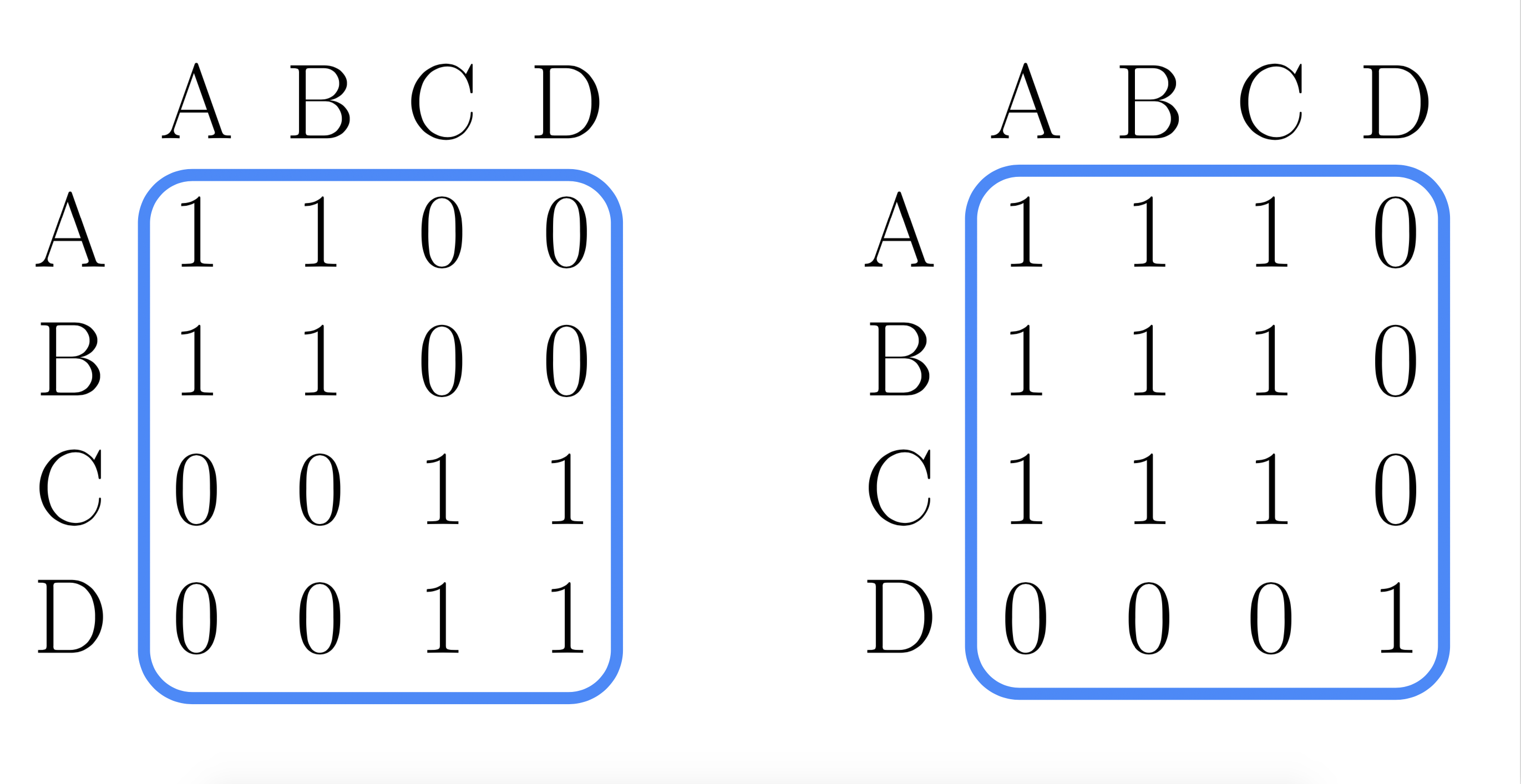
- Step2: Consensus matrix:
Average of all the partitions
10.1.2.4.5 Tools for consensus clustering: SC3
10.2 Clustering example
library(pcaMethods)
library(SC3)
library(scater)
library(SingleCellExperiment)
library(pheatmap)
library(mclust)
library(igraph)
library(scran)
10.2.1 Example 1. Graph-based clustering (deng dataset)
To illustrate clustering of scRNA-seq data, we consider the Deng dataset of
cells from developing mouse embryo (Deng et al. 2014). We have preprocessed the
dataset and created a SingleCellExperiment object in advance. We have also
annotated the cells with the cell types identified in the original publication
(it is the cell_type2 column in the colData slot).
First, we build a \(K\)-NN graph with a package function from scran. The most important decision of building a graph is the choice of \(K\), of which there is no standard rule. In general, we can think of it as an indication of the desired cluster size. If \(K\) is too small, a genuine cluster might be split into parts, while if \(K\) is too large, clusters might not thoroughly separated.
deng5 <- buildSNNGraph(deng, k = 5)
deng15 <- buildSNNGraph(deng, k = 15)
deng25 <- buildSNNGraph(deng, k = 25)
par(mfrow=c(1,3))
plot(deng5, vertex.size = 4, vertex.label = NA)
title("5-NN" ,line = -33, cex.main = 3)
plot(deng15, vertex.size = 4, vertex.label = NA)
title("15-NN" ,line = -33, cex.main = 3)
plot(deng25, vertex.size = 4, vertex.label = NA)
title("25-NN" ,line = -33, cex.main = 3)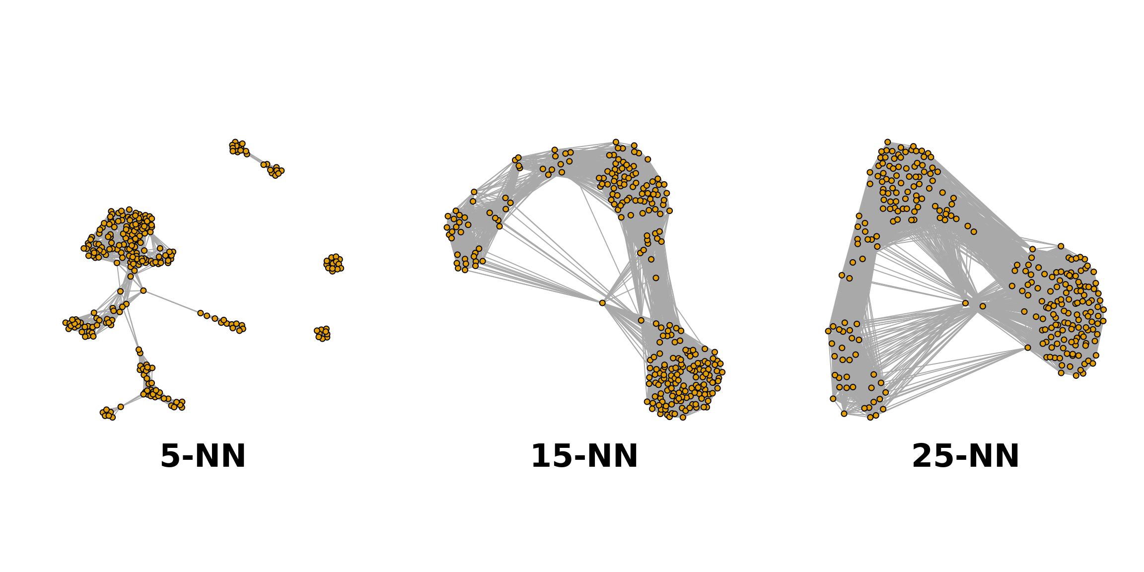
Perform Louvain clustering:
cl <- igraph::cluster_louvain(deng15)$membership
colData(deng)$cl <- factor(cl)
mclust::adjustedRandIndex(colData(deng)$cell_type2, colData(deng)$cl)
## [1] 0.4197754Reaches very high similarity with the labels provided in the original paper.
However, it tend to merge small clusters into larger ones.
##             cl
##               1  2  3
##   16cell     49  0  1
##   4cell       0 14  0
##   8cell      36  0  1
##   early2cell  0  8  0
##   earlyblast  0  0 43
##   late2cell   0 10  0
##   lateblast   0  0 30
##   mid2cell    0 12  0
##   midblast    0  0 60
##   zy          0  4  0
10.2.2 Example 2. Graph-based clustering (segerstolpe dataset)
muraro <- readRDS("data/pancreas/muraro.rds")
## PCA
var.fit <- suppressWarnings(trendVar(muraro, parametric=TRUE, use.spikes=F))
muraro <- suppressWarnings(denoisePCA(muraro, technical=var.fit$trend))
dim(reducedDim(muraro, "PCA"))
## [1] 2126 5## Build graph and clustering
gr <- buildSNNGraph(muraro, use.dimred="PCA", k = 30)
cl <- igraph::cluster_louvain(gr)$membership
colData(muraro)$cl <- factor(cl)
mclust::adjustedRandIndex(colData(muraro)$cell_type1, colData(muraro)$cl)## [1] 0.4845618## cl
## 1 2 3 4 5 6 7 8 9
## acinar 0 0 0 0 0 0 218 0 1
## alpha 202 306 274 5 15 9 1 0 0
## beta 1 0 0 5 195 21 2 220 4
## delta 0 0 0 0 18 174 0 1 0
## ductal 0 0 0 215 0 1 7 3 19
## endothelial 0 0 0 0 0 0 0 0 21
## epsilon 0 0 0 0 0 3 0 0 0
## gamma 1 0 1 0 0 97 2 0 0
## mesenchymal 0 0 0 1 0 0 0 0 79
## unclear 0 0 0 4 0 0 0 0 010.2.3 Example 3. SC3
Let’s run SC3 clustering on the Deng data. The advantage of the SC3 is that it can directly ingest a SingleCellExperiment object.
SC3 can estimate a number of clusters:
## Estimating k...## [1] 6Next we run SC3 (we also ask it to calculate biological properties of the clusters):
## Setting SC3 parameters...## Calculating distances between the cells...## Performing transformations and calculating eigenvectors...## Performing k-means clustering...## Calculating consensus matrix...## Calculating biology...SC3 result consists of several different outputs (please look in (Kiselev et al. 2017) and SC3 vignette for more details). Here we show some of them:
Consensus matrix:
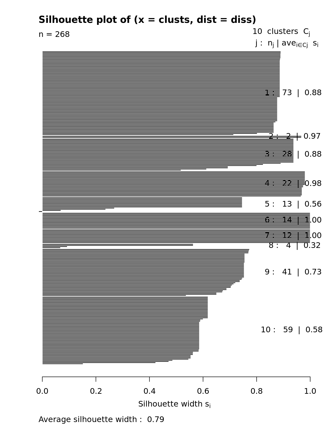
Silhouette plot:
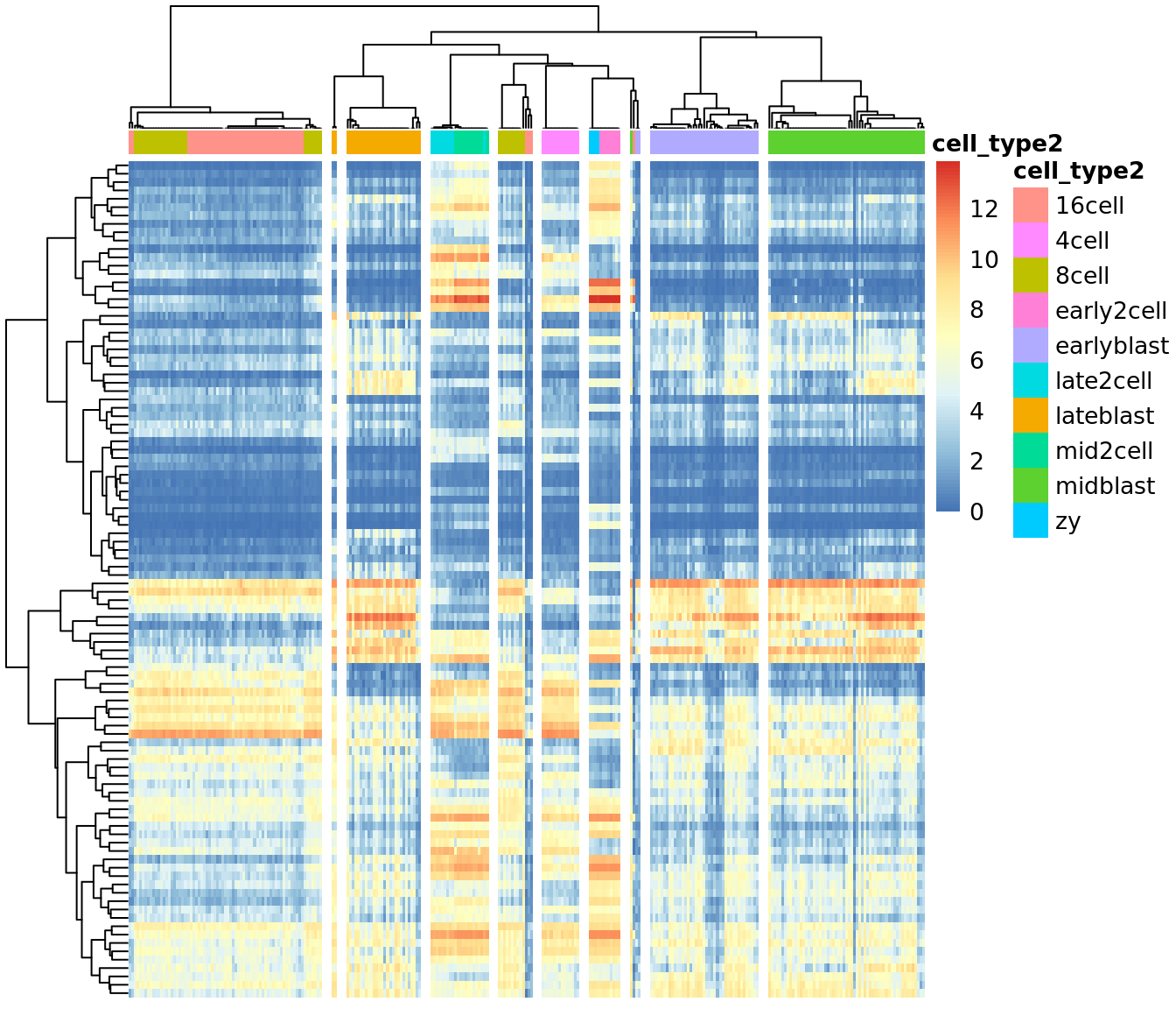
Heatmap of the expression matrix:
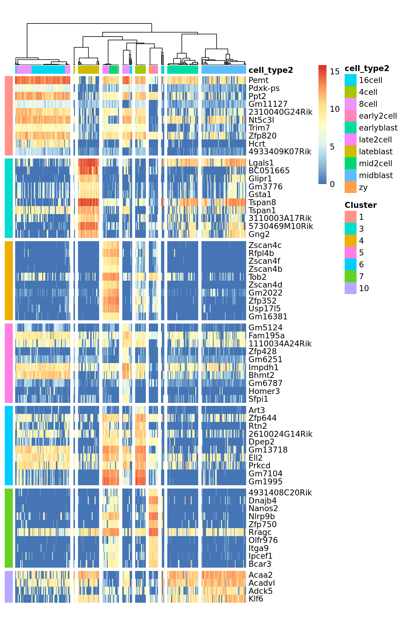
Identified marker genes:
PCA plot with highlighted SC3 clusters:
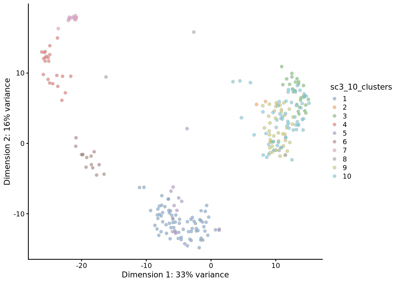
Compare the results of SC3 clustering with the original publication cell type labels:
## [1] 0.7804189Note SC3 can also be run in an interactive Shiny session:
This command will open SC3 in a web browser.
Note Due to direct calculation of distances SC3 becomes very slow when the number of cells is \(>5000\). For large datasets containing up to \(10^5\) cells we recomment using Seurat (see chapter 16).
10.3 An alternative to clustering: Automatic cell annotation
10.3.1 SingleR
10.3.1.1 Methodology
- Step1. Find variable gene
1-1. For every gene, obtain median grouped by label.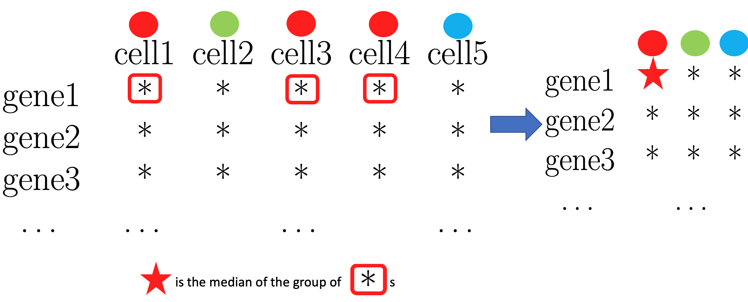
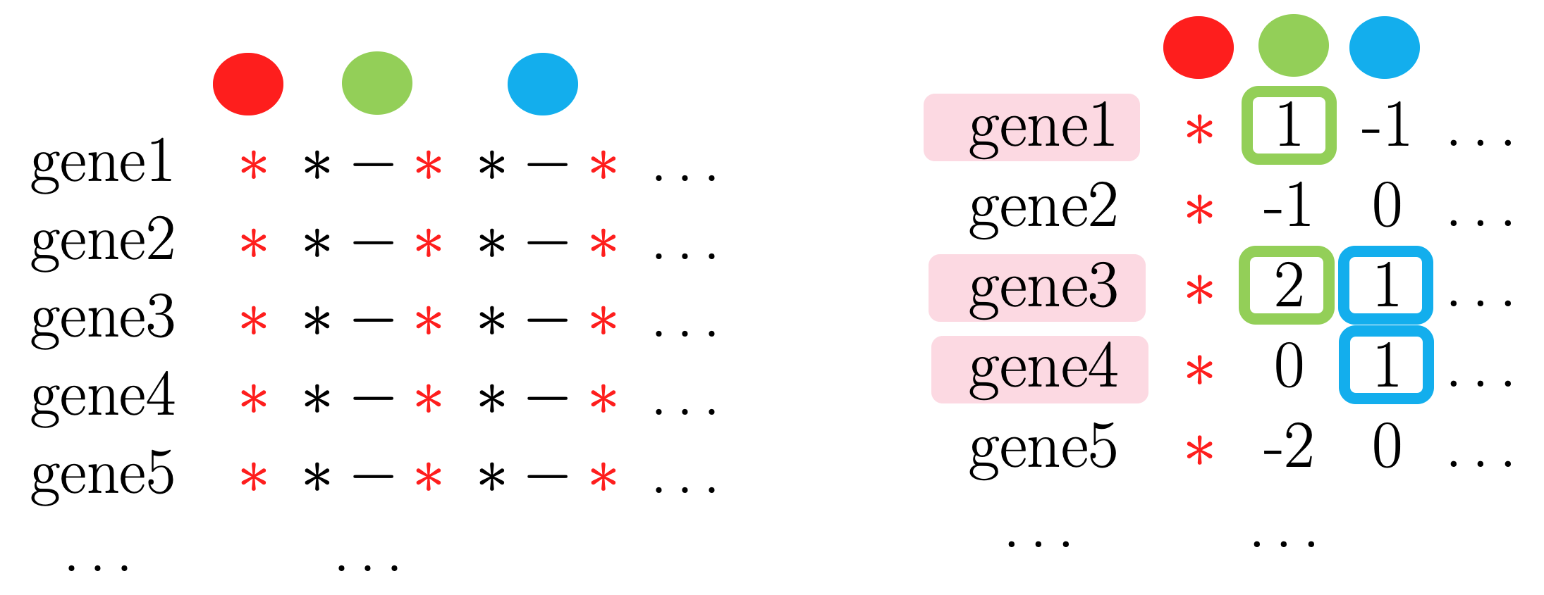
- Step2. Spearman’s correlation
Spearman’s correlation \(\in [-1, 1]\) is a measure of the strength of a linear or monotonic relationship between paired data.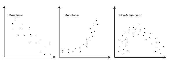
- Step3. Scoring
We want to know how each cell in the test data is correlated to the labels in the reference data, instead of each reference cell. So we take the correlations of a cell in the test data with all the cells with a certain label in the reference data, and summarize them into one number or a score, in SingleR, the default is to take the \(80\%\) quantile.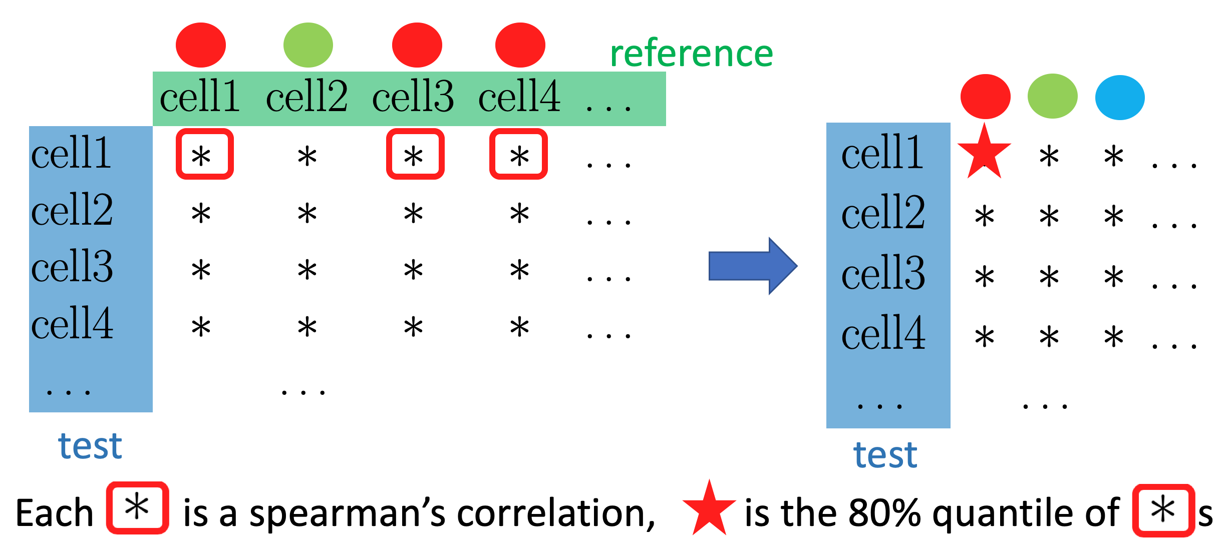
- Step4. Fine tuning
We stop here and assign each cell with label that score the highest, actually, if we set the argumentfine.tune = FALSE, that is exactly what the package functionSingleRdoes. But there is one more question, what if the second highest score is very close to the highest? say, 1, 1, 1, 9.5, 10.SingleRset a threshold to define how close is “very close”, the default is 0.05. For (only) the cells that falls into this category, it goes back to Step2.
10.3.1.2 Example
(Note: SingleR is not yet available in the released version of Bioconductor. It will be possible to run it as shown once the next Bioconductor release is made in late October.)
library(scRNAseq)
library(SingleR)
segerstolpe <- readRDS("data/pancreas/segerstolpe.rds")
sceM <- suppressMessages(MuraroPancreasData())
sceM <- sceM[,!is.na(sceM$label)]
sceM <- logNormCounts(sceM)
## find common gene
rownames(sceM) <- gsub("__.*","",rownames(sceM))
common <- intersect(rownames(sceM), rownames(segerstolpe))
sceM <- sceM[common,]
segerstolpe <- segerstolpe[common,]
## Prepare reference
out <- pairwiseTTests(logcounts(sceM), sceM$label, direction="up")
markers <- getTopMarkers(out$statistics, out$pairs, n=10)
## Annotation
pred <- SingleR(test=segerstolpe, ref=sceM, labels=sceM$label, genes=markers)
## View result
plotScoreHeatmap(pred, show.labels = TRUE,  annotation_col=data.frame(
  row.names=rownames(pred)))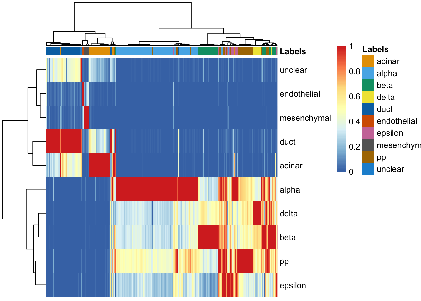
10.3.2 scmap
## Load data
segerstolpe <- readRDS("data/pancreas/segerstolpe.rds")  # test
library(scRNAseq)
sceM <- readRDS("data/pancreas/muraro.rds") # reference
rownames(sceM) <- gsub("__.*","",rownames(sceM))
Select the most informative features (genes) using the dropout feature selection method. By default select 500 features.
library(scmap)
rowData(sceM)$feature_symbol <- rownames(sceM)
sceM <- selectFeatures(sceM, suppress_plot = TRUE)
Index of a reference dataset is created by finding the median gene expression for each cluster. First, chop the total of 500 features into \(M = 50\) chuncks/ low-dimensional subspace. Second, cluster each chunk into \(k = \sqrt{N}\) clusters, where \(N\) is the number of cells.
By default scmap uses the cell_type1 column of the colData slot in the
reference to identify clusters.
The function indexCluster writes the scmap_cluster_index item of the meta data slot of the reference dataset sceM.
This step has two outputs:
## [1] "subcentroids" "subclusters"subcentroidsreturns cluster centers:
## 50 chunks## The dimension of cluster centers in each chunk: 10 46subclusterscontains information about which cluster (label) the cells belong to
## [1] 50 2126## D28.1_1 D28.1_13 D28.1_15 D28.1_17 D28.1_2
## [1,] 8 14 5 3 3
## [2,] 15 40 8 35 4
## [3,] 7 43 21 1 20
## [4,] 27 42 34 27 30
## [5,] 45 38 4 41 36Projection: Once the scmap-cell indexes have been generated we can use them to project the test dataset.
scmapCell_results <- scmapCell(
  projection = segerstolpe,
  index_list = list(
    sceM = metadata(sceM)$scmap_cell_index
  ) )
names(scmapCell_results)
## [1] "sceM"The cells matrix contains the top 10 (scmap default) cell IDs of the cells
of the reference dataset that a given cell of the projection dataset is closest
to:
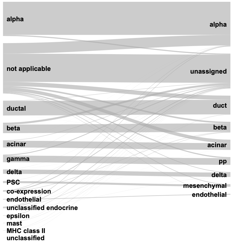
## [1] 10 3514Cell annotation: If cell cluster annotation is available for the reference datasets, scmap-cell can also annotate the cells from the projection dataset using the labels of the reference. It does so by looking at the top 3 nearest neighbours (scmap default) and if they all belong to the same cluster in the reference and their maximum similarity is higher than a threshold (0.5 is the scmap default), then a projection cell is assigned to the corresponding reference cluster:
Plot result Compare the annotated result with the original label in the
segerstolpe dataset.
10.3.3 sessionInfo()
References
Blondel, Vincent D, Jean-Loup Guillaume, Renaud Lambiotte, and Etienne Lefebvre. 2008. “Fast Unfolding of Communities in Large Networks.” Journal of Statistical Mechanics: Theory and Experiment 2008 (10). IOP Publishing: P10008.
Deng, Q., D. Ramskold, B. Reinius, and R. Sandberg. 2014. “Single-Cell RNA-Seq Reveals Dynamic, Random Monoallelic Gene Expression in Mammalian Cells.” Science 343 (6167). American Association for the Advancement of Science (AAAS): 193–96. https://doi.org/10.1126/science.1245316.
Freytag, Saskia, Luyi Tian, Ingrid Lönnstedt, Milica Ng, and Melanie Bahlo. 2018. “Comparison of Clustering Tools in R for Medium-Sized 10x Genomics Single-Cell Rna-Sequencing Data.” F1000Research 7. Faculty of 1000 Ltd.
Good, Benjamin H, Yves-Alexandre De Montjoye, and Aaron Clauset. 2010. “Performance of Modularity Maximization in Practical Contexts.” Physical Review E 81 (4). APS: 046106.
Kiselev, Vladimir Yu, Kristina Kirschner, Michael T Schaub, Tallulah Andrews, Andrew Yiu, Tamir Chandra, Kedar N Natarajan, et al. 2017. “SC3: Consensus Clustering of Single-Cell RNA-Seq Data.” Nat Meth 14 (5). Springer Nature: 483–86. https://doi.org/10.1038/nmeth.4236.
Newman, Mark EJ, and Michelle Girvan. 2004. “Finding and Evaluating Community Structure in Networks.” Physical Review E 69 (2). APS: 026113.
Traag, Vincent A, Ludo Waltman, and Nees Jan van Eck. 2019. “From Louvain to Leiden: Guaranteeing Well-Connected Communities.” Scientific Reports 9. Nature Publishing Group.