11 Trajectory inference
library(SingleCellExperiment)
library(TSCAN)
library(M3Drop)
library(monocle)
library(destiny)
library(scater)
library(ggplot2)
library(ggthemes)
library(ggbeeswarm)
library(corrplot)
library(Polychrome)
library(slingshot)
library(SLICER)
library(ouija)
set.seed(1)
In many situations, one is studying a process where cells change continuously. This includes, for example, many differentiation processes taking place during development: following a stimulus, cells will change from one cell-type to another. Ideally, we would like to monitor the expression levels of an individual cell over time. Unfortunately, such monitoring is not possible with scRNA-seq since the cell is lysed (destroyed) when the RNA is extracted.
Instead, we must sample at multiple time-points and obtain snapshots of the gene expression profiles. Since some of the cells will proceed faster along the differentiation than others, each snapshot may contain cells at varying points along the developmental progression. We use statistical methods to order the cells along one or more trajectories which represent the underlying developmental trajectories, this ordering is referred to as “pseudotime”.
In this chapter we will consider five different tools: TSCAN,Slingshot,Monocle and some off-the-shelf methods like PCA,
for ordering cells according to their pseudotime development.
To illustrate the methods we will be using a dataset on mouse embryonic
development (Deng et al. 2014). The dataset consists of 268 cells from 10 different
time-points of early mouse development. In this case, there is no need for
pseudotime alignment since the cell labels provide information about the
development trajectory. Thus, the labels allow us to establish a ground truth so
that we can evaluate and compare the different methods.
A recent benchmarking paper by Saelens et al (Saelens et al. 2019) provides a detailed summary of the various computational methods for trajectory inference from single-cell transcriptomics (Saelens et al. 2019). They discuss 45 tools and evaluate them across various aspects including accuracy, scalability, and usability.
The following figures from the paper summarise several key aspects and some of the features of the tools being evaluated:
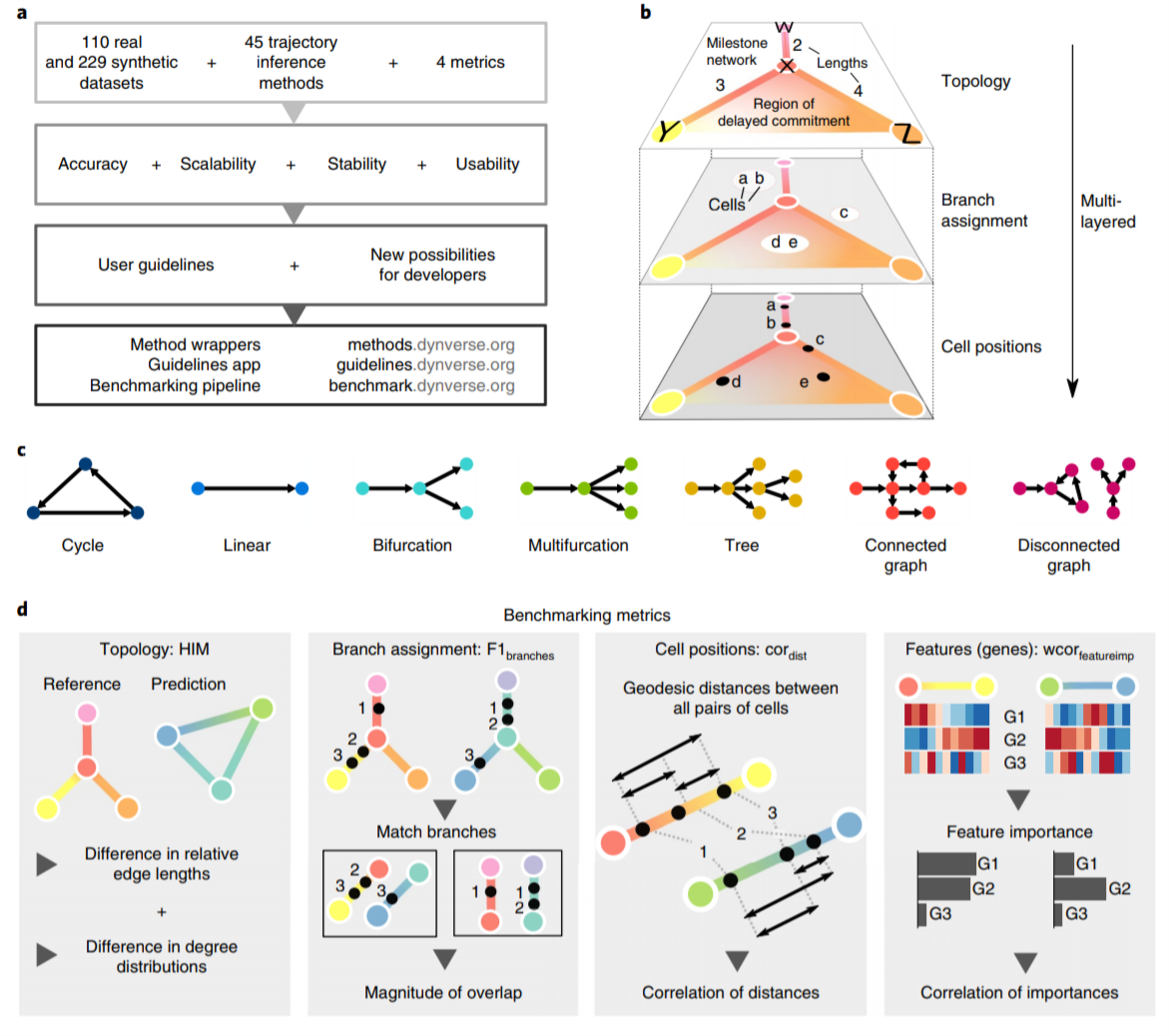
Figure 2.3: Overview of several key aspects of the evaluation (Fig. 1 from Saelens et al, 2019).
The Characterizatics of the 45 TI tools:
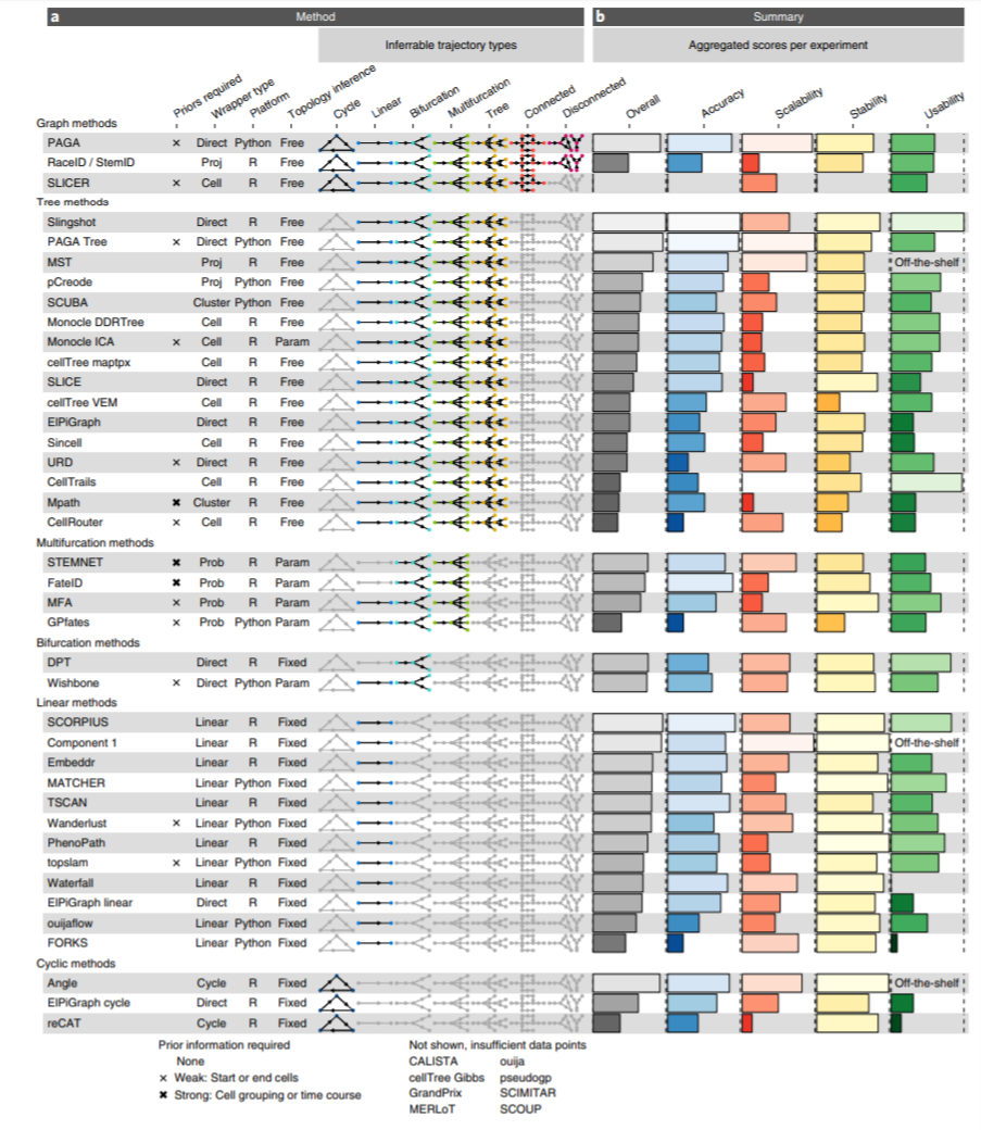
Figure 2.4: Characterization of trajectory inference methods for single-cell transcriptomics data (Fig. 2 from Saelens et al, 2019).
The detailed evaluation results of the 45 TI tools:
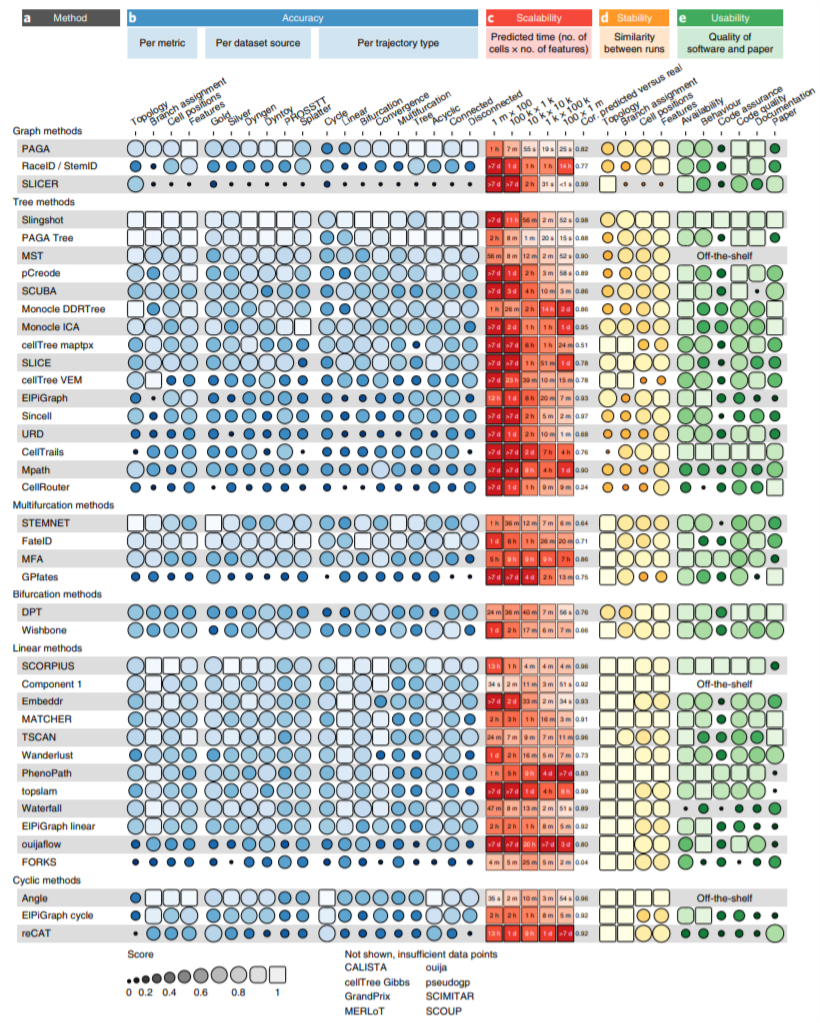
Figure 2.5: Detailed results of the four main evaluation criteria: accuracy, scalability, stability and usability of trajectory inference methods for single-cell transcriptomics data (Fig. 3 from Saelens et al, 2019).
11.1 First look at Deng data
Let us take a first look at the Deng(Deng et al. 2014) data, without yet applying sophisticated pseudotime methods. As the plot below shows, simple PCA does a very good job of displaying the structure in these data. It is only once we reach the blast cell types (“earlyblast”, “midblast”, “lateblast”) that PCA struggles to separate the distinct cell types.
deng_SCE <- readRDS("data/deng/deng-reads.rds")

deng_SCE$cell_type2 <- factor(
    deng_SCE$cell_type2,
    levels = c("zy", "early2cell", "mid2cell", "late2cell",
                        "4cell", "8cell", "16cell", "earlyblast",
                        "midblast", "lateblast")
)
cellLabels <- deng_SCE$cell_type2
deng <- counts(deng_SCE)
colnames(deng) <- cellLabels

deng_SCE <- scater::runPCA(deng_SCE,ncomponent = 5)

## change color Palette with library(Polychrome)

set.seed(723451) # for reproducibility
my_color <- createPalette(10, c("#010101", "#ff0000"), M=1000)
names(my_color) <- unique(as.character(deng_SCE$cell_type2))

pca_df <- data.frame(PC1 = reducedDim(deng_SCE,"PCA")[,1],
                     PC2 = reducedDim(deng_SCE,"PCA")[,2],
                     cell_type2 = deng_SCE$cell_type2)

ggplot(data = pca_df)+geom_point(mapping = aes(x = PC1, y = PC2, colour = cell_type2))+
  scale_colour_manual(values = my_color)+theme_classic()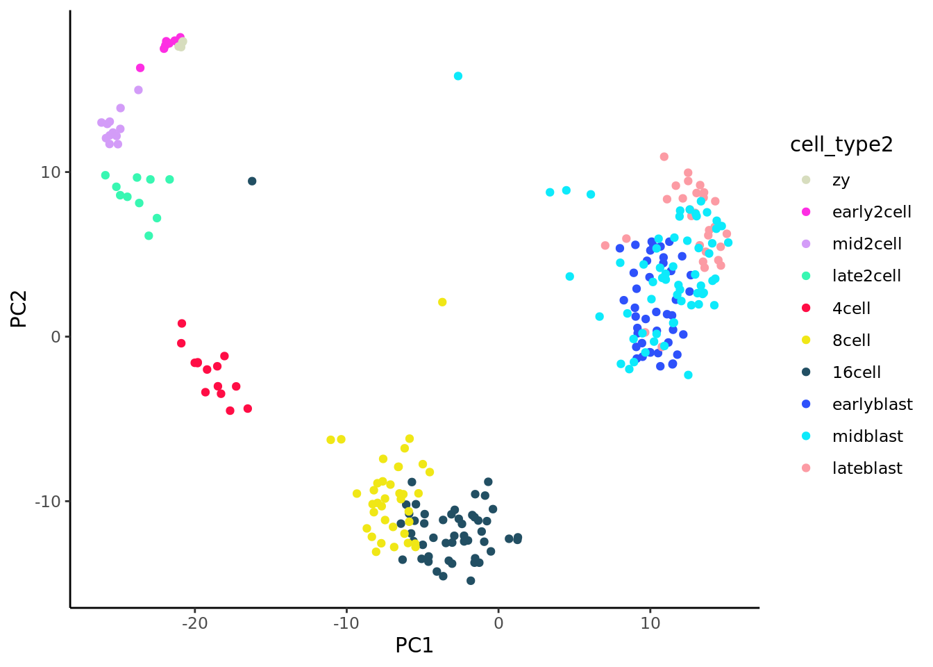
PCA, here, provides a useful baseline for assessing different pseudotime methods. For a very naive pseudotime we can just take the co-ordinates of the first principal component.
#deng_SCE$PC1 <- reducedDim(deng_SCE, "PCA")[,1]

ggplot(pca_df, aes(x = PC1, y = cell_type2,
                              colour = cell_type2)) +
    geom_quasirandom(groupOnX = FALSE) +
    scale_colour_manual(values = my_color) + theme_classic() +
    xlab("First principal component") + ylab("Timepoint") +
    ggtitle("Cells ordered by first principal component")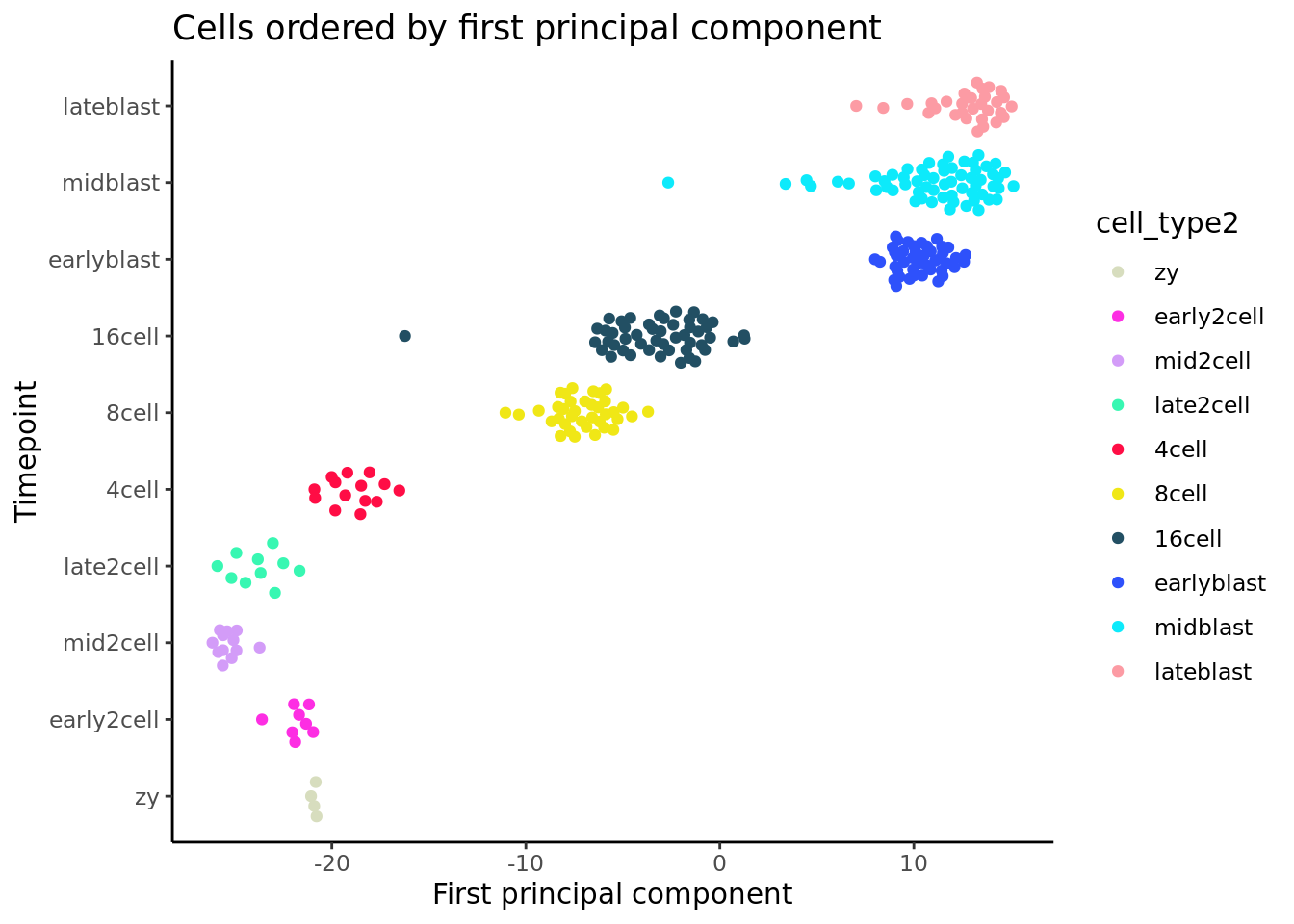
As the plot above shows, PC1 struggles to correctly order cells early and late in the developmental timecourse, but overall does a relatively good job of ordering cells by developmental time.
Can bespoke pseudotime methods do better than naive application of PCA?
11.2 TSCAN
TSCAN (Ji and Ji 2019) combines clustering with pseudotime analysis. First it clusters the cells using mclust, which is based on a mixture of normal distributions. Then it builds a minimum spanning tree to connect the clusters. The branch of this tree that connects the largest number of clusters is the main branch which is used to determine pseudotime.
Note From a connected graph with weighted edges, MST is the tree structure that connects all the nodes in a way that has the minimum total edge weight. The trajectory inference methods that use MST is based on the idea that nodes (cells/clusters of cells) and their connections represent the geometric shape of the data cloud in a two-dimenension space.
First we will try to use all genes to order the cells.
procdeng <- TSCAN::preprocess(counts(deng_SCE))

colnames(procdeng) <- 1:ncol(deng_SCE)

dengclust <- TSCAN::exprmclust(procdeng, clusternum = 10)

TSCAN::plotmclust(dengclust)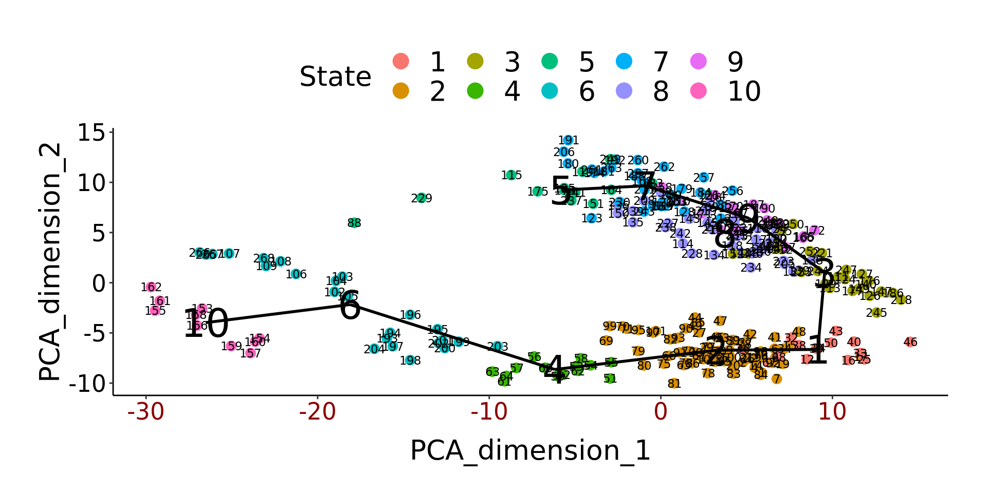
dengorderTSCAN <- TSCAN::TSCANorder(dengclust, orderonly = FALSE)
pseudotime_order_tscan <- as.character(dengorderTSCAN$sample_name)
deng_SCE$pseudotime_order_tscan <- NA
deng_SCE$pseudotime_order_tscan[as.numeric(dengorderTSCAN$sample_name)] <-
    dengorderTSCAN$Pseudotime
Frustratingly, TSCAN only provides pseudotime values for 221 of 268 cells, silently returning missing values for non-assigned cells.
Again, we examine which timepoints have been assigned to each state:
##  [1] late2cell late2cell late2cell late2cell late2cell late2cell late2cell
##  [8] late2cell late2cell late2cell
## 10 Levels: zy early2cell mid2cell late2cell 4cell 8cell ... lateblastggplot(as.data.frame(colData(deng_SCE)),
aes(x = pseudotime_order_tscan,
y = cell_type2, colour = cell_type2)) +
geom_quasirandom(groupOnX = FALSE) +
scale_color_manual(values = my_color) + theme_classic() +
xlab("TSCAN pseudotime") + ylab("Timepoint") +
ggtitle("Cells ordered by TSCAN pseudotime")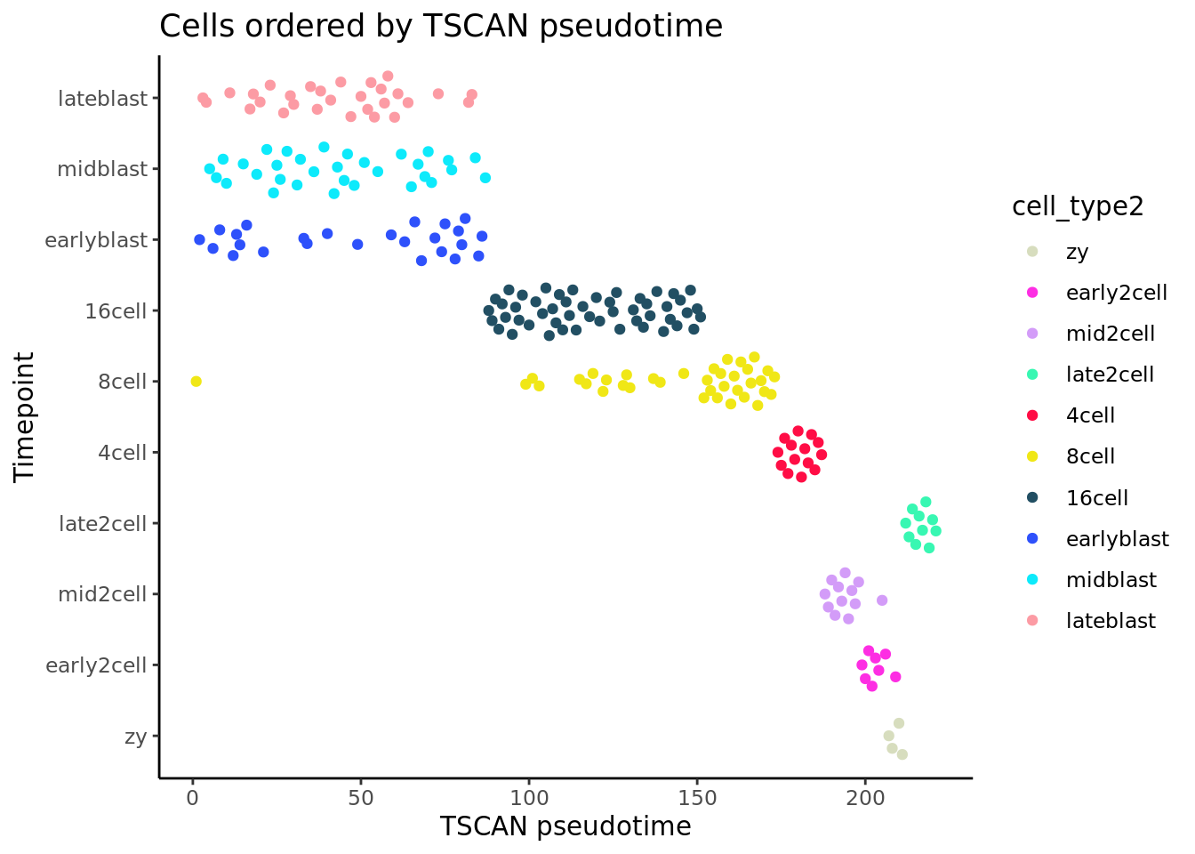
TSCAN gets the development trajectory the “wrong way around”, in the sense that later pseudotime values correspond to early timepoints and vice versa. This is not inherently a problem (it is easy enough to reverse the ordering to get the intuitive interpretation of pseudotime), but overall it would be a stretch to suggest that TSCAN performs better than PCA on this dataset. (As it is a PCA-based method, perhaps this is not entirely surprising.)
Exercise 1 Compare results for different numbers of clusters (clusternum).
11.3 Slingshot
Slingshot (Street et al. 2018) is a single-cell lineage inference tool, it can work with datasets with multiple branches. Slingshot has two stages: 1) the inference of the global lineage structure using MST on clustered data points and 2) the inference of pseudotime variables for cells along each lineage by fitting simultaneous ‘principal curves’ across multiple lineages.
Slingshot’s first stage uses a cluster-based MST to stably identify the key elements of the global lineage structure, i.e., the number of lineages and where they branch. This allows us to identify novel lineages while also accommodating the use of domain-specific knowledge to supervise parts of the tree (e.g., terminal cellular states). For the second stage, we propose a novel method called simultaneous principal curves, to fit smooth branching curves to these lineages, thereby translating the knowledge of global lineage structure into stable estimates of the underlying cell-level pseudotime variable for each lineage.
Slingshot had consistently performing well across different datasets as reported by Saelens et al, let’s have a run for the deng dataset. It is recommended by Slingshot to run in a reduced dimensions.
__Note_ Principal curves are smooth one-dimensional curves that pass through the middle of a p-dimensional data set, providing a nonlinear summary of the data. They are nonparametric, and their shape is suggested by the data (Hastie et al)(Hastie and Stuetzle 1989).
## runing slingshot

deng_SCE <- slingshot(deng_SCE, clusterLabels = 'cell_type2',reducedDim = "PCA",
                      allow.breaks = FALSE)
## Using diagonal covariance matrix## Min. 1st Qu. Median Mean 3rd Qu. Max. NA's
## 0.00 52.19 59.81 60.34 81.60 85.72 55## get lineages inferred by slingshot
lnes <- getLineages(reducedDim(deng_SCE,"PCA"),
deng_SCE$cell_type2)## Using diagonal covariance matrix## $Lineage1
## [1] "zy" "early2cell" "mid2cell" "late2cell" "4cell"
## [6] "16cell" "midblast" "earlyblast"
##
## $Lineage2
## [1] "zy" "early2cell" "mid2cell" "late2cell" "4cell"
## [6] "16cell" "midblast" "lateblast"
##
## $Lineage3
## [1] "zy" "early2cell" "mid2cell" "late2cell" "4cell"
## [6] "16cell" "8cell"## plot the lineage overlay on the orginal PCA plot
plot(reducedDims(deng_SCE)$PCA, col = my_color[as.character(deng_SCE$cell_type2)],
pch=16,
asp = 1)
legend("bottomleft",legend = names(my_color[levels(deng_SCE$cell_type2)]),
fill = my_color[levels(deng_SCE$cell_type2)])
lines(SlingshotDataSet(deng_SCE), lwd=2, type = 'lineages', col = c("black"))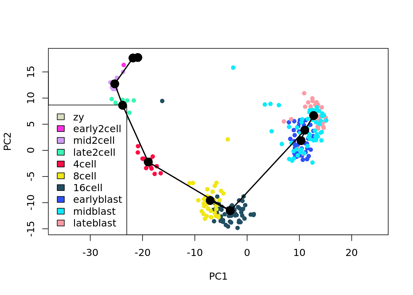
## Plotting the pseudotime inferred by slingshot by cell types

slingshot_df <- data.frame(colData(deng_SCE))

ggplot(slingshot_df, aes(x = slingPseudotime_1, y = cell_type2,
                              colour = cell_type2)) +
    geom_quasirandom(groupOnX = FALSE) + theme_classic() +
    xlab("First Slingshot pseudotime") + ylab("cell type") +
    ggtitle("Cells ordered by Slingshot pseudotime")+scale_colour_manual(values = my_color)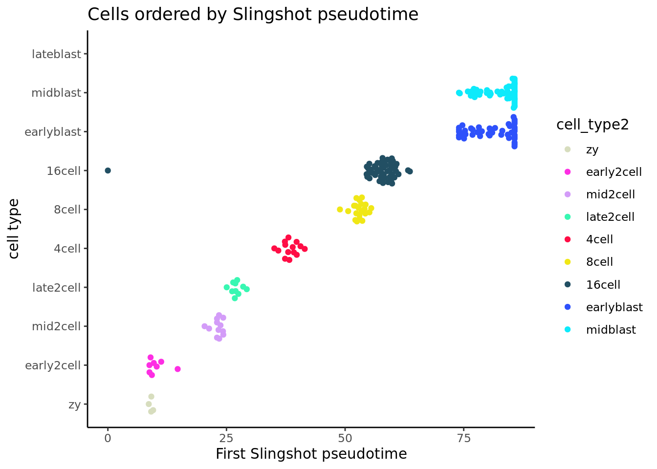
ggplot(slingshot_df, aes(x = slingPseudotime_2, y = cell_type2,
                              colour = cell_type2)) +
    geom_quasirandom(groupOnX = FALSE) + theme_classic() +
    xlab("Second Slingshot pseudotime") + ylab("cell type") +
    ggtitle("Cells ordered by Slingshot pseudotime")+scale_colour_manual(values = my_color)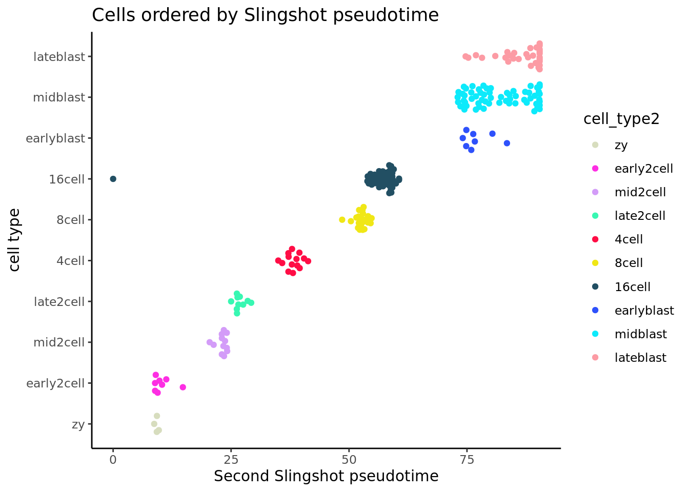
ggplot(slingshot_df, aes(x = slingPseudotime_1, y = slingPseudotime_2,
                              colour = cell_type2)) +
    geom_quasirandom(groupOnX = FALSE) + theme_classic() +
    xlab("First Slingshot pseudotime") + ylab("Second Slingshot pseudotime") +
    ggtitle("Cells ordered by Slingshot pseudotime")+scale_colour_manual(values = my_color)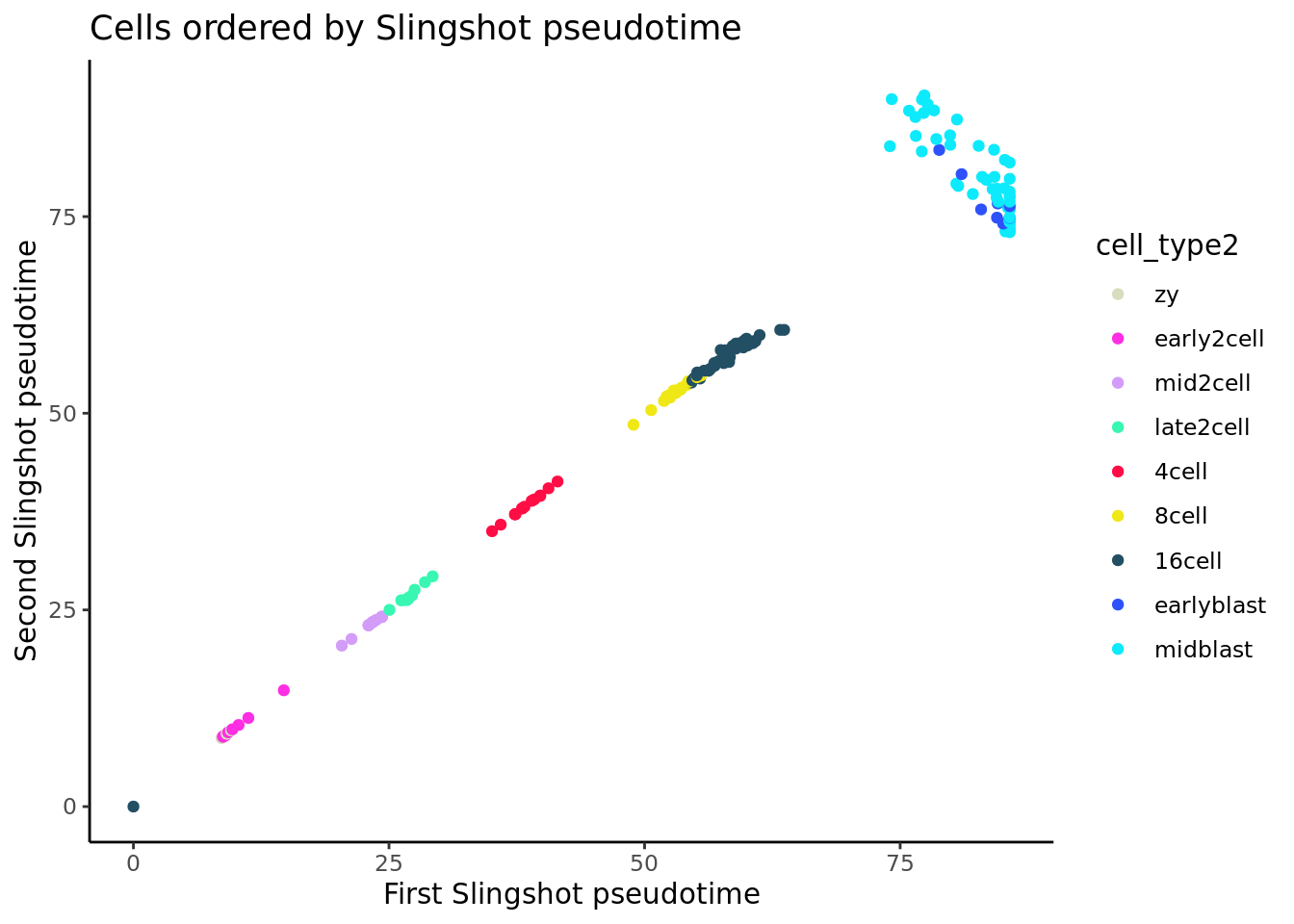
#
# ggplot(slingshot_df, aes(x = slingPseudotime_1, y = slingPseudotime_2,
#                               colour = slingPseudotime_3)) +
#     geom_point() + theme_classic() +
#     xlab("First Slingshot pseudotime") + ylab("Second Slingshot pseudotime") +
#     ggtitle("Cells ordered by Slingshot pseudotime")+facet_wrap(.~cell_type2)
Note You can also supply a start and an end cluster to slingshot.
Comments Did you notice the ordering of clusters in the lineage prediced for 16cells state? There is an outlier-like cell in the 16cell group, find the outlier and remove it, then re-run Slingshot.
11.3.1 GAM general additive model for identifying temporally expressed genes
After running slingshot, an interesting next step may be to find genes that change their expression over the course of development. We demonstrate one possible method for this type of analysis on the 100 most variable genes. We will regress each gene on the pseudotime variable we have generated, using a general additive model (GAM). This allows us to detect non-linear patterns in gene expression.
library(gam)
t <- deng_SCE$slingPseudotime_1

# for time, only look at the 100 most variable genes
Y <- log1p(assay(deng_SCE,"logcounts"))

var100 <- names(sort(apply(Y,1,var),decreasing = TRUE))[1:100]
Y <- Y[var100,]

# fit a GAM with a loess term for pseudotime
gam.pval <- apply(Y,1,function(z){
    d <- data.frame(z=z, t=t)
    suppressWarnings({
      tmp <- gam(z ~ lo(t), data=d)
    })
    p <- summary(tmp)[3][[1]][2,3]
    p
})

## Plot the top 100 genes' expression

topgenes <- names(sort(gam.pval, decreasing = FALSE))[1:100]

heatdata <- assays(deng_SCE)$logcounts[topgenes, order(t, na.last = NA)]
heatclus <- deng_SCE$cell_type2[order(t, na.last = NA)]

heatmap(heatdata, Colv = NA,
        ColSideColors = my_color[heatclus],cexRow = 1,cexCol = 1)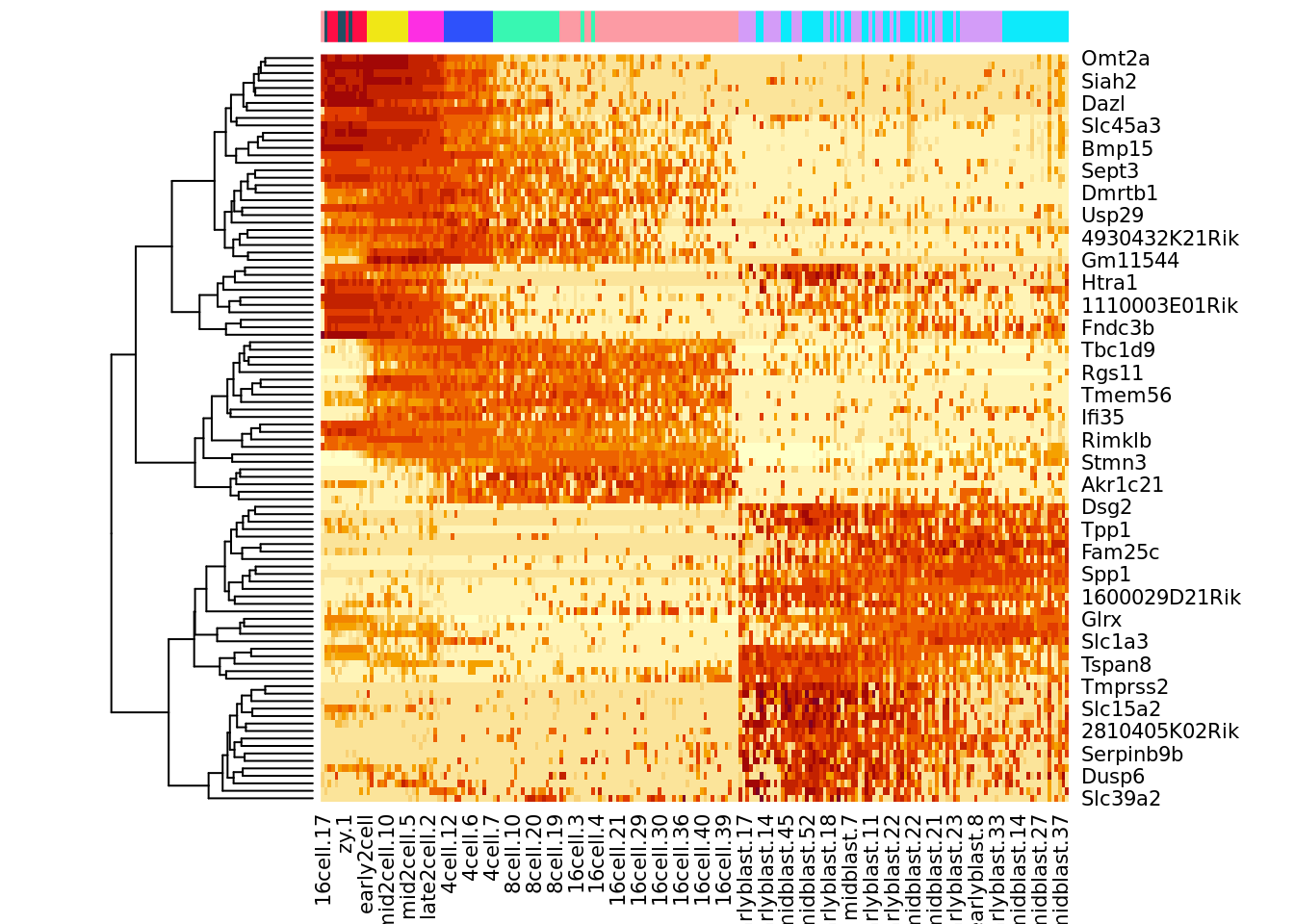
11.4 Monocle
The original Monocle (Trapnell et al. 2014) method skips the clustering stage of TSCAN and directly builds a
minimum spanning tree on a reduced dimension representation (using ‘ICA’) of the
cells to connect all cells. Monocle then identifies the longest path
in this tree as the main branch and uses this to determine pseudotime. Priors are required such as start/end state and the number of branching events.
If the data contains diverging trajectories (i.e. one cell type differentiates into two different cell-types), monocle can identify these. Each of the resulting forked paths is defined as a separate cell state.
11.4.1 Monocle 2
Monocle 2 (Qiu et al. 2017) uses a different approach, with dimensionality reduction and ordering performed by reverse
graph embedding (RGE), allowing it to detect branching events in an unsupervised manner. RGE, a machine-learning strategy, learns a ‘principal graph’ to describe the single-cell dataset. RGE also learns the mapping function of data points on the trajectory back to the original high dimentional space simutaneously. In doing so, it aims to position the latent points in the lower dimension space (along the trajectory) while also ensuring their corresponding
positions in the input dimension are ‘neighbors’.
There are different ways of implementing the RGE framework, Monocle 2 uses DDRTree(Discriminative dimensionality reduction via learning a tree) by default.
DDRTree learns latent points and the projection of latent points to the points in original input space, which is equivalent to “dimension reduction”. In addition, it simutanously learns ‘principal graph’ for K-means soft clustered centroids for the latent points. Principal graph is the spanning tree of those centroids.
DDRTree returns a principal tree of the centroids of cell clusters in low dimension, pseudotime is derived for individual cells by calculating geomdestic distance of their projections onto the tree from the root (user-defined or arbitrarily assigned).
Note Informally, a principal graph is like a principal curve which passes through the ‘middle’ of a data set but is allowed to have branches.
library(monocle)
#d <- deng_SCE[m3dGenes,]
## feature selection
deng <- counts(deng_SCE)

m3dGenes <- as.character(
    M3DropFeatureSelection(deng)$Gene
)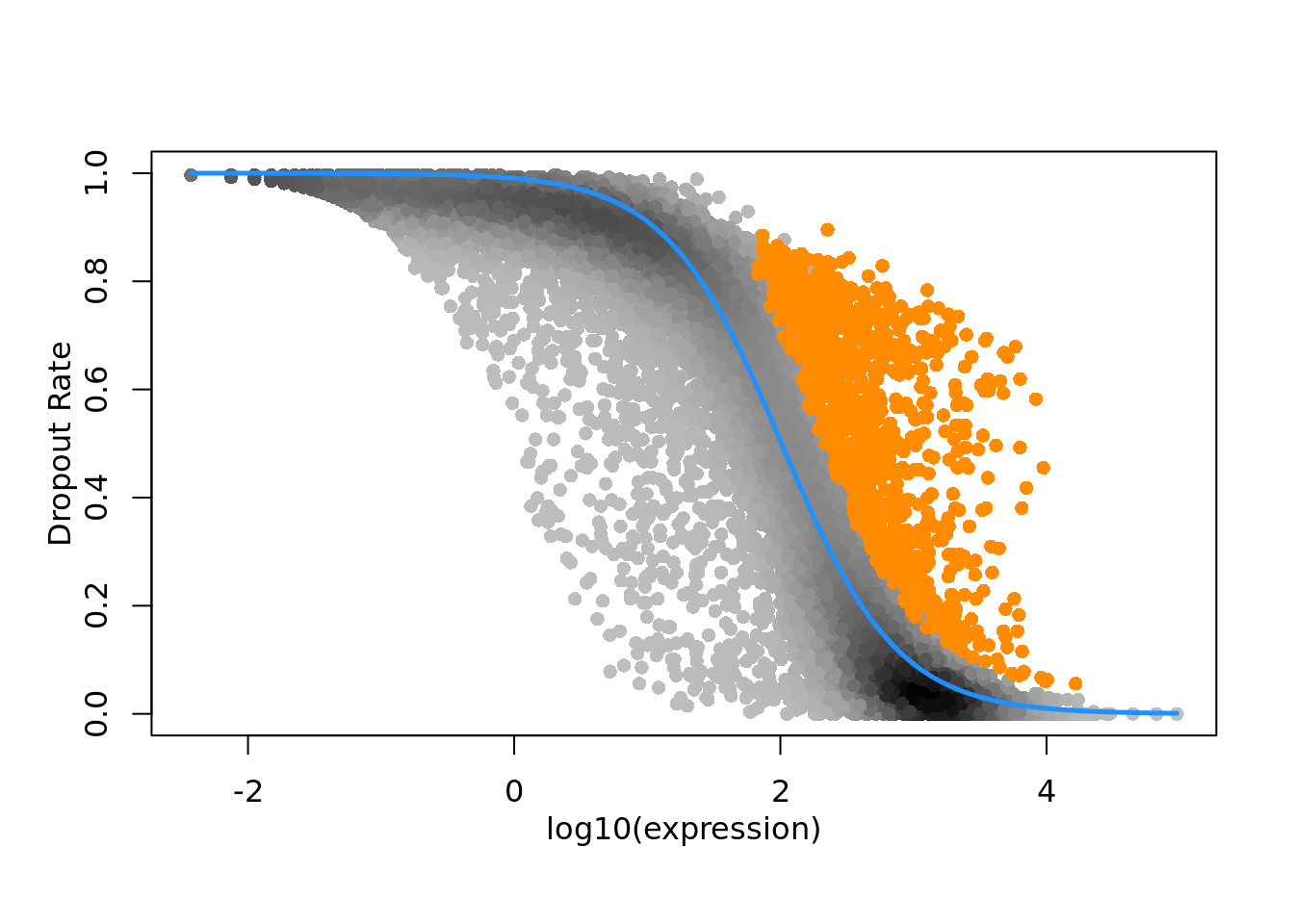
d <- deng_SCE[which(rownames(deng_SCE) %in% m3dGenes), ]
d <- d[!duplicated(rownames(d)), ]

colnames(d) <- 1:ncol(d)
geneNames <- rownames(d)
rownames(d) <- 1:nrow(d)
pd <- data.frame(timepoint = cellLabels)
pd <- new("AnnotatedDataFrame", data=pd)
fd <- data.frame(gene_short_name = geneNames)
fd <- new("AnnotatedDataFrame", data=fd)

dCellData <- newCellDataSet(counts(d), phenoData = pd, featureData = fd)
#
dCellData <- setOrderingFilter(dCellData, which(geneNames %in% m3dGenes))
dCellData <- estimateSizeFactors(dCellData)
dCellDataSet <- reduceDimension(dCellData,reduction_method = "DDRTree", pseudo_expr = 1)
dCellDataSet <- orderCells(dCellDataSet, reverse = FALSE)
plot_cell_trajectory(dCellDataSet)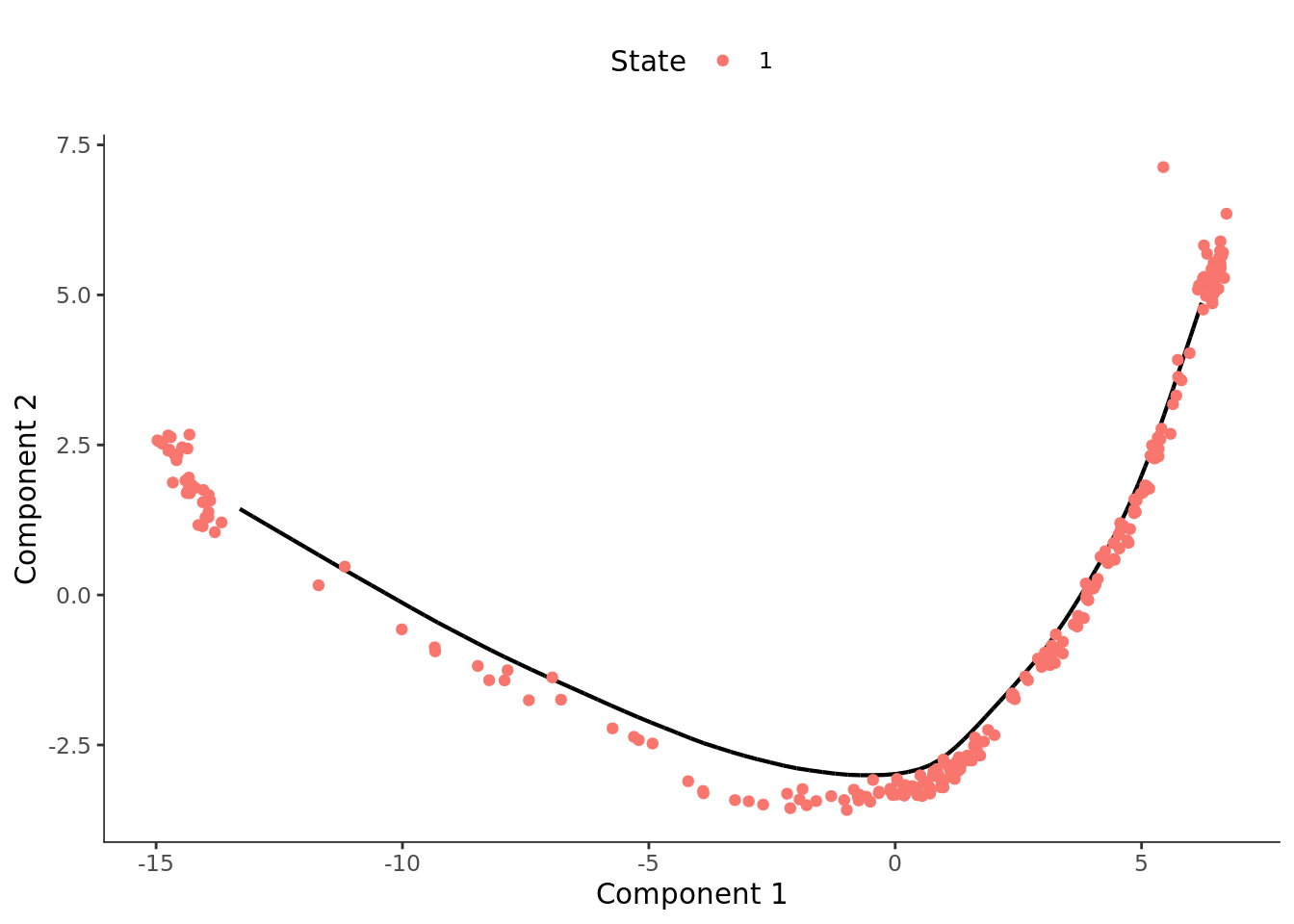
# Store the ordering
pseudotime_monocle2 <-
    data.frame(
        Timepoint = phenoData(dCellDataSet)$timepoint,
        pseudotime = phenoData(dCellDataSet)$Pseudotime,
        State = phenoData(dCellDataSet)$State
    )
rownames(pseudotime_monocle2) <- 1:ncol(d)
pseudotime_order_monocle <-
    rownames(pseudotime_monocle2[order(pseudotime_monocle2$pseudotime), ])
Note check other available methods for ?reduceDimension
We can again compare the inferred pseudotime to the known sampling timepoints.
deng_SCE$pseudotime_monocle2 <- pseudotime_monocle2$pseudotime

ggplot(as.data.frame(colData(deng_SCE)),
       aes(x = pseudotime_monocle2,
           y = cell_type2, colour = cell_type2)) +
    geom_quasirandom(groupOnX = FALSE) +
    scale_color_manual(values = my_color) + theme_classic() +
    xlab("monocle2 pseudotime") + ylab("Timepoint") +
    ggtitle("Cells ordered by monocle2 pseudotime")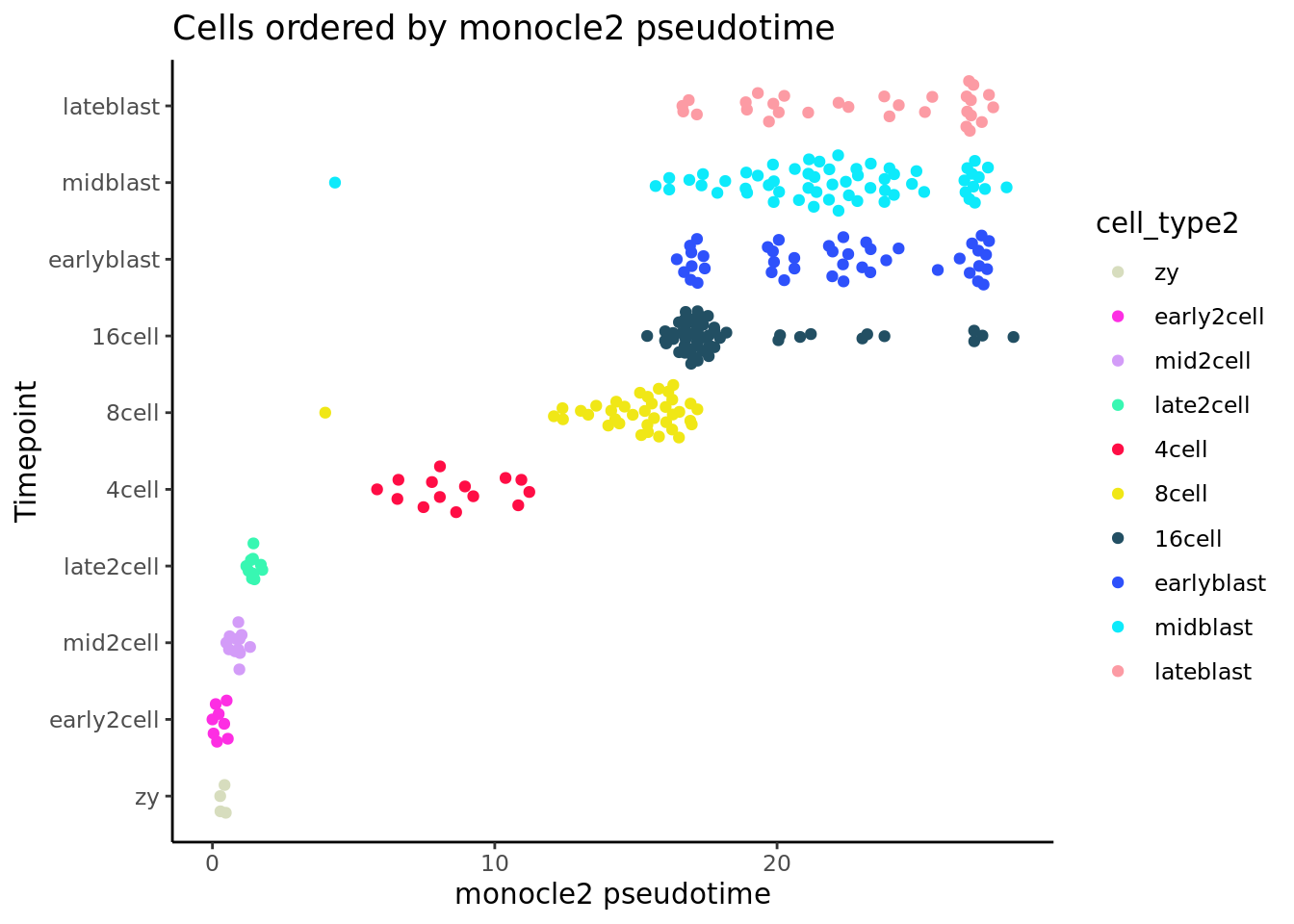
Monocle 2 performs pretty well on these cells.
11.4.2 Monocle 3
Monocle3(Cao et al. 2019) is the updated single-cell analysis toolkit for analysing large datasets. Monocle 3 is designed for use with absolute transcript counts (e.g. from UMI experiments). It first does dimension reduction with UMAP, then it clusters the cells with Louvain/Leiden algorithms and merge adjacent groups into supergroup, and finaly resovles the trajectories individual cells can take during development within each supergroup.
In short, Monocle3 uses UMAP to construct a initial trajectory inference and refines it with learning principal graph.
It builds KNN graph in the UMAP dimensions and runs Louvain/Leiden algorithms on the KNN graph to derive communities; edges are drawn to connect communities that have more links (Partitioned Approximate Graph Abstraction (PAGA) graph). Each component of the PAGA graph is passed to the next step which is learning principal graph based on the SimplePPT algorithm. The pseudotime is calculated for individual cells by projecting the cells to their nearest point on the principal graph edge and measure geodestic distance along of principal points to the closest of their root nodes.
##
## Attaching package: 'monocle3'
## The following objects are masked from 'package:monocle':
##
## plot_genes_in_pseudotime, plot_genes_violin,
## plot_pc_variance_explained## The following objects are masked from 'package:Biobase':
##
## exprs, fData, fData<-, pData, pData<-gene_meta <- rowData(deng_SCE)
#gene_metadata must contain a column verbatim named 'gene_short_name' for certain functions.
gene_meta$gene_short_name <- rownames(gene_meta)
cds <- new_cell_data_set(expression_data = counts(deng_SCE),
cell_metadata = colData(deng_SCE),
gene_metadata = gene_meta)
## Step 1: Normalize and pre-process the data
cds <- preprocess_cds(cds,num_dim = 5)
plot_pc_variance_explained(cds)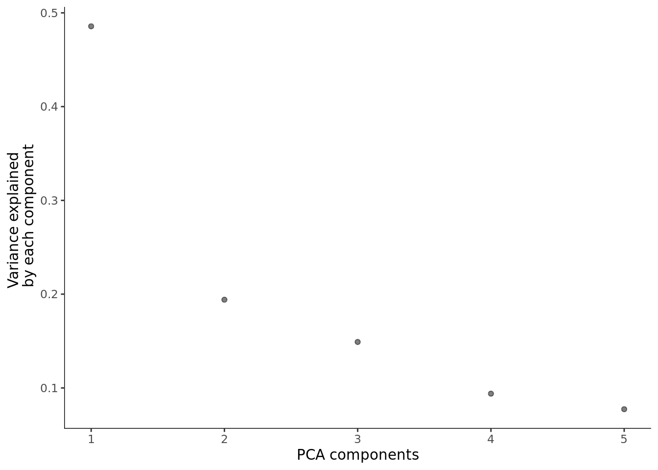
## No preprocess_method specified, using preprocess_method = 'PCA'## Step 4: Cluster the cells
cds <- cluster_cells(cds)
## change the clusters
## cds@clusters$UMAP$clusters <- deng_SCE$cell_type2
## Step 5: Learn a graph
cds <- learn_graph(cds,use_partition = TRUE)
## Step 6: Order cells
cds <- order_cells(cds, root_cells = c("zy","zy.1","zy.2","zy.3") )
plot_cells(cds, color_cells_by="cell_type2", graph_label_size = 4, cell_size = 2,
group_label_size = 6)+ scale_color_manual(values = my_color) 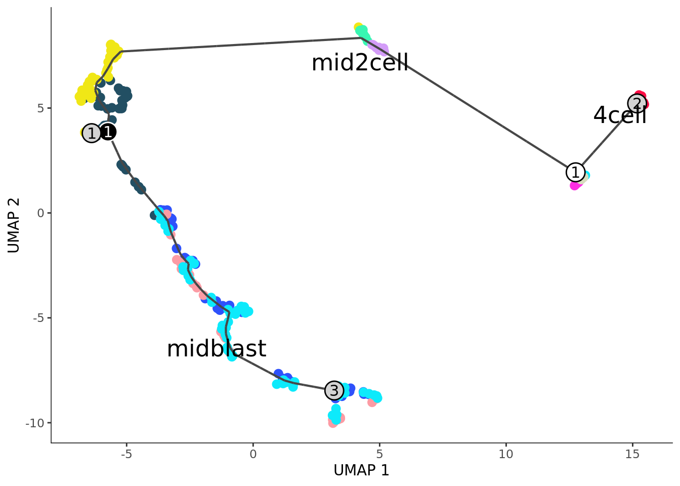
plot_cells(cds,  graph_label_size = 6, cell_size = 1,
           color_cells_by="pseudotime",
           group_label_size = 6)
## Cells aren't colored in a way that allows them to be grouped.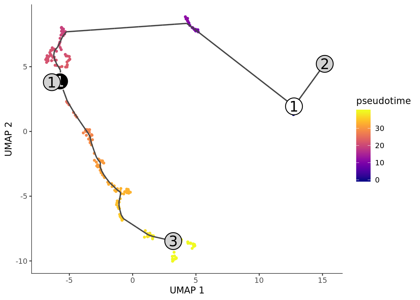
pdata_cds <- pData(cds)
pdata_cds$pseudotime_monocle3 <- monocle3::pseudotime(cds)

ggplot(as.data.frame(pdata_cds),
       aes(x = pseudotime_monocle3,
           y = cell_type2, colour = cell_type2)) +
    geom_quasirandom(groupOnX = FALSE) +
    scale_color_manual(values = my_color) + theme_classic() +
    xlab("monocle3 pseudotime") + ylab("Timepoint") +
    ggtitle("Cells ordered by monocle3 pseudotime")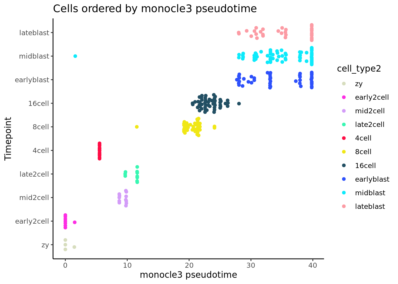
It did not work well for our small Smart-seq2 dataset.
11.4.3 Diffusion maps
Diffusion maps were introduced by Ronald Coifman and Stephane Lafon(Coifman and Lafon 2006), and the underlying idea is to assume that the data are samples from a diffusion process. The method infers the low-dimensional manifold by estimating the eigenvalues and eigenvectors for the diffusion operator related to the data.
Angerer et al(Angerer et al. 2016) have applied the diffusion maps concept to the analysis of single-cell RNA-seq data to create an R package called destiny.
We will take the ranko prder of cells in the first diffusion map component as “diffusion map pseudotime” here.
deng <- logcounts(deng_SCE)
colnames(deng) <- cellLabels
dm <- DiffusionMap(t(deng))

tmp <- data.frame(DC1 = eigenvectors(dm)[,1],
                  DC2 = eigenvectors(dm)[,2],
                  Timepoint = deng_SCE$cell_type2)
ggplot(tmp, aes(x = DC1, y = DC2, colour = Timepoint)) +
    geom_point() +  scale_color_manual(values = my_color) +
    xlab("Diffusion component 1") +
    ylab("Diffusion component 2") +
    theme_classic()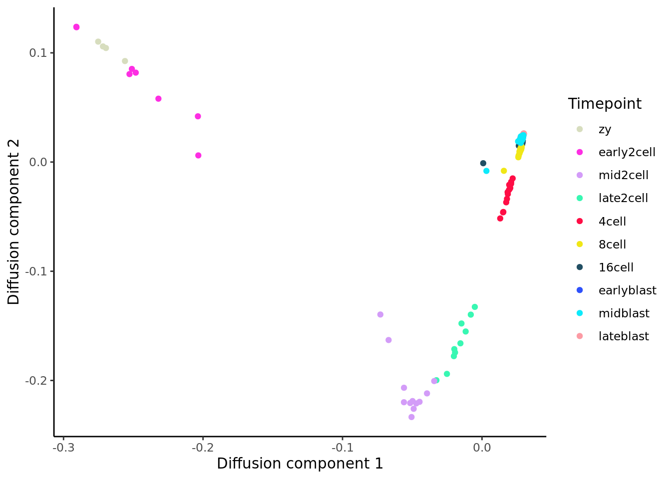
deng_SCE$pseudotime_diffusionmap <- rank(eigenvectors(dm)[,1])

ggplot(as.data.frame(colData(deng_SCE)),
       aes(x = pseudotime_diffusionmap,
           y = cell_type2, colour = cell_type2)) +
    geom_quasirandom(groupOnX = FALSE) +
    scale_color_manual(values = my_color)  + theme_classic() +
    xlab("Diffusion map pseudotime (first diffusion map component)") +
    ylab("Timepoint") +
    ggtitle("Cells ordered by diffusion map pseudotime")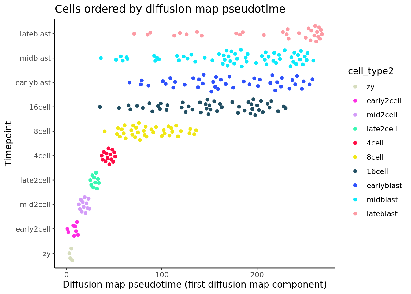
Like the other methods, using the first diffusion map component from destiny as pseudotime does a good job at ordering the early time-points (if we take high values as “earlier” in developement), but it is unable to distinguish the later ones.
Exercise 2 Do you get a better resolution between the later time points by considering additional eigenvectors?
Exercise 3 How does the ordering change if you only use the genes identified by M3Drop?
11.5 Other methods
11.5.1 SLICER
The SLICER(Welch, Hartemink, and Prins 2016) method is an algorithm for constructing trajectories that
describe gene expression changes during a sequential biological
process, just as Monocle and TSCAN are. SLICER is designed to capture
highly nonlinear gene expression changes, automatically select genes
related to the process, and detect multiple branch and loop features
in the trajectory (Welch, Hartemink, and Prins 2016). The SLICER R package is available
from its GitHub repository and
can be installed from there using the devtools package.
We use the select_genes function in SLICER to automatically select
the genes to use in builing the cell trajectory. The function uses
“neighbourhood variance” to identify genes that vary smoothly, rather
than fluctuating randomly, across the set of cells. Following this, we
determine which value of “k” (number of nearest neighbours) yields an embedding that
most resembles a trajectory. Then we estimate the locally linear
embedding of the cells.
library("lle")
slicer_genes <- select_genes(t(deng))
k <- select_k(t(deng[slicer_genes,]), kmin = 30, kmax=60)
## finding neighbours
## calculating weights
## computing coordinates
## finding neighbours
## calculating weights
## computing coordinates
## finding neighbours
## calculating weights
## computing coordinates
## finding neighbours
## calculating weights
## computing coordinates
## finding neighbours
## calculating weights
## computing coordinates
## finding neighbours
## calculating weights
## computing coordinates
## finding neighbours
## calculating weights
## computing coordinates## finding neighbours
## calculating weights
## computing coordinatesreducedDim(deng_SCE, "LLE") <- slicer_traj_lle
plot_df <- data.frame(slicer1 = reducedDim(deng_SCE, "LLE")[,1],
slicer2 = reducedDim(deng_SCE, "LLE")[,2],
cell_type2 = deng_SCE$cell_type2)
ggplot(data = plot_df)+geom_point(mapping = aes(x = slicer1,
y = slicer2,
color = cell_type2))+
scale_color_manual(values = my_color)+ xlab("LLE component 1") +
ylab("LLE component 2") +
ggtitle("Locally linear embedding of cells from SLICER")+
theme_classic()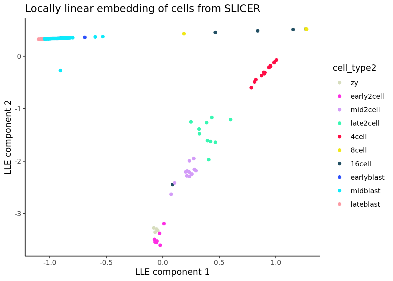
With the locally linear embedding computed we can construct a k-nearest neighbour graph that is fully connected. This plot displays a (yellow) circle for each cell, with the cell ID number overlaid in blue. Here we show the graph computed using 10 nearest neighbours. Here, SLICER appears to detect one major trajectory with one branch.
slicer_traj_graph <- conn_knn_graph(slicer_traj_lle, 10)
plot(slicer_traj_graph, main = "Fully connected kNN graph from SLICER")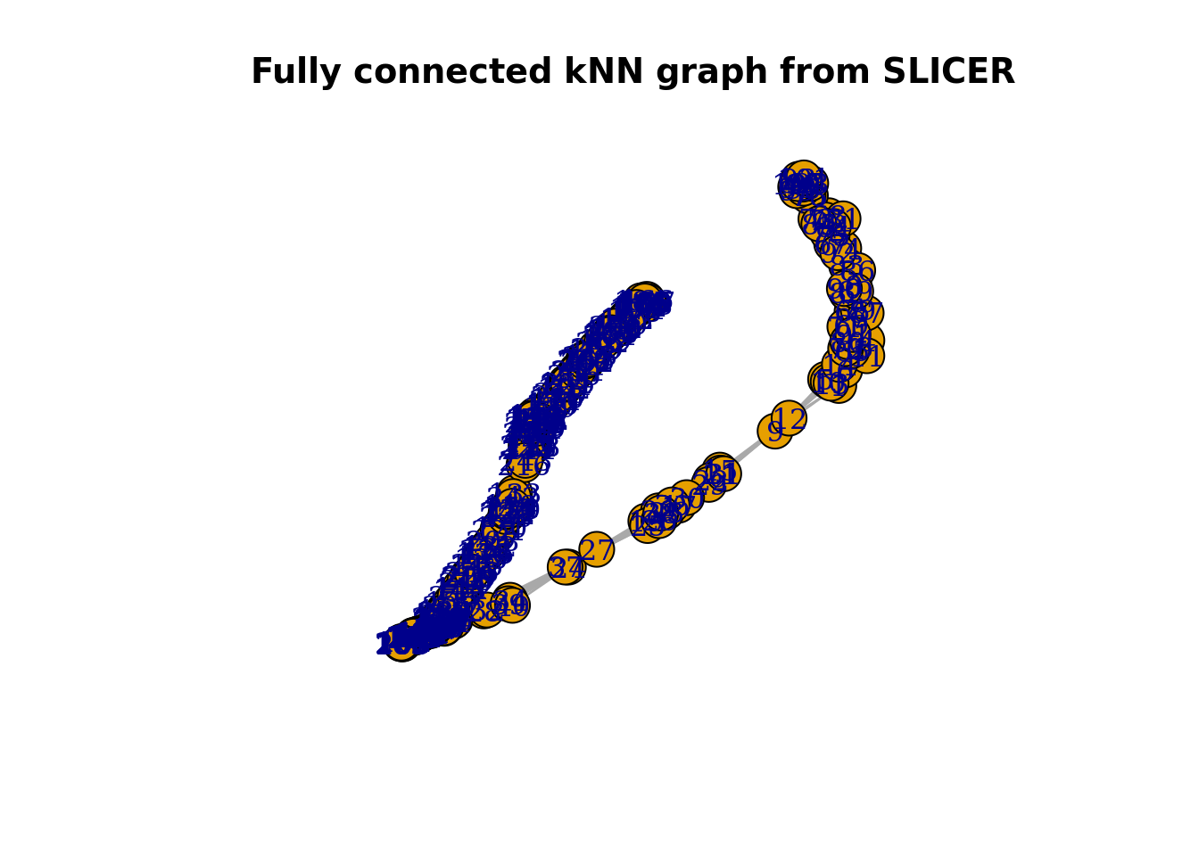
From this graph we can identify “extreme” cells that are candidates for start/end cells in the trajectory.
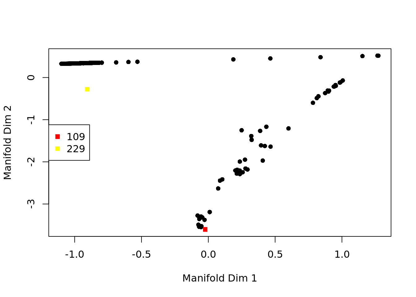
Having defined a start cell we can order the cells in the estimated pseudotime.
pseudotime_order_slicer <- cell_order(slicer_traj_graph, start)
branches <- assign_branches(slicer_traj_graph, start)

pseudotime_slicer <-
    data.frame(
        Timepoint = cellLabels,
        pseudotime = NA,
        State = branches
    )
pseudotime_slicer$pseudotime[pseudotime_order_slicer] <-
    1:length(pseudotime_order_slicer)
deng_SCE$pseudotime_slicer <- pseudotime_slicer$pseudotime
We can again compare the inferred pseudotime to the known sampling timepoints. SLICER does not provide a pseudotime value per se, just an ordering of cells.
ggplot(as.data.frame(colData(deng_SCE)),
       aes(x = pseudotime_slicer,
           y = cell_type2, colour = cell_type2)) +
    geom_quasirandom(groupOnX = FALSE) +
    scale_color_manual(values = my_color) + theme_classic() +
    xlab("SLICER pseudotime (cell ordering)") +
    ylab("Timepoint") +
    theme_classic()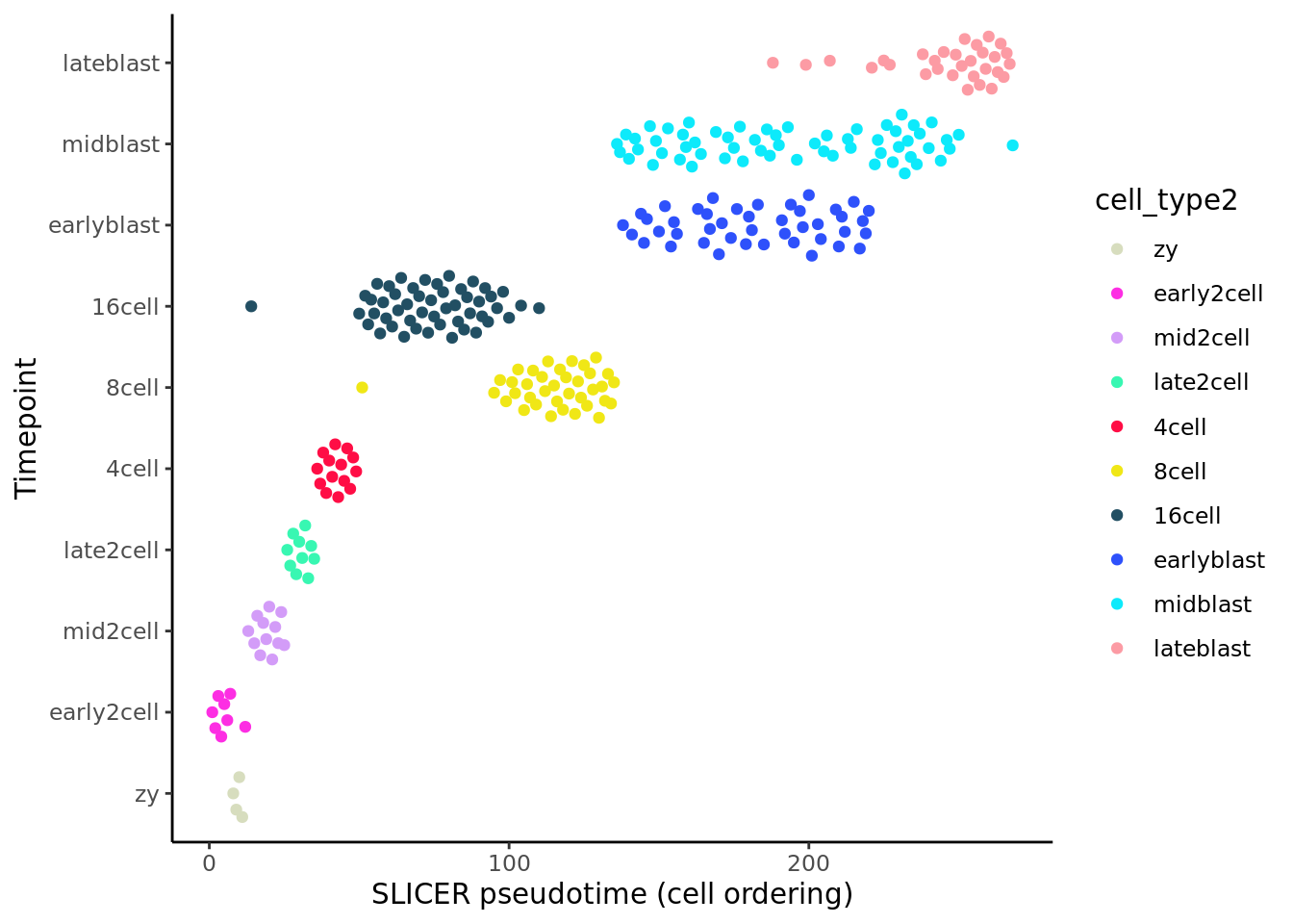
Like the previous method, SLICER (Welch, Hartemink, and Prins 2016) here provides a good ordering for the early time points. It places “16cell” cells before “8cell” cells, but provides better ordering for blast cells than many of the earlier methods.
Exercise 4 How do the results change for different k? (e.g. k = 5) What about changing the number of nearest neighbours in
the call to conn_knn_graph?
Exercise 5 How does the ordering change if you use a different set of genes from those chosen by SLICER (e.g. the genes identified by M3Drop)?
11.5.2 Ouija
Ouija (http://kieranrcampbell.github.io/ouija/) takes a different approach from the pseudotime estimation methods we have looked at so far. Earlier methods have all been “unsupervised”, which is to say that apart from perhaps selecting informative genes we do not supply the method with any prior information about how we expect certain genes or the trajectory as a whole to behave.
Ouija, in contrast, is a probabilistic framework that allows for interpretable learning of single-cell pseudotimes using only small panels of marker genes. This method:
- infers pseudotimes from a small number of marker genes letting you understand why the pseudotimes have been learned in terms of those genes;
- provides parameter estimates (with uncertainty) for interpretable gene regulation behaviour (such as the peak time or the upregulation time);
- has a Bayesian hypothesis test to find genes regulated before others along the trajectory;
- identifies metastable states, ie discrete cell types along the continuous trajectory.
We will supply the following marker genes to Ouija (with timepoints where they are expected to be highly expressed):
- Early timepoints: Dazl, Rnf17, Sycp3, Nanog, Pou5f1, Fgf8, Egfr, Bmp5, Bmp15
- Mid timepoints: Zscan4b, Foxa1, Prdm14, Sox21
- Late timepoints: Creb3, Gpx4, Krt8, Elf5, Eomes, Cdx2, Tdgf1, Gdf3
With Ouija we can model genes as either exhibiting monotonic up or down regulation (known as switch-like behaviour), or transient behaviour where the gene briefly peaks. By default, Ouija assumes all genes exhibit switch-like behaviour (the authors assure us not to worry if we get it wrong - the noise model means incorrectly specifying a transient gene as switch-like has minimal effect).
Here we can “cheat” a little and check that our selected marker genes do actually identify different timepoints of the differentiation process.
ouija_markers_down <- c("Dazl", "Rnf17", "Sycp3", "Fgf8",
                        "Egfr", "Bmp5", "Bmp15", "Pou5f1")
ouija_markers_up <- c("Creb3", "Gpx4", "Krt8", "Elf5", "Cdx2",
                      "Tdgf1", "Gdf3", "Eomes")
ouija_markers_transient <- c("Zscan4b", "Foxa1", "Prdm14", "Sox21")
ouija_markers <- c(ouija_markers_down, ouija_markers_up,
                   ouija_markers_transient)
plotExpression(deng_SCE, ouija_markers, x = "cell_type2", colour_by = "cell_type2") +
    theme(axis.text.x = element_text(angle = 60, hjust = 1))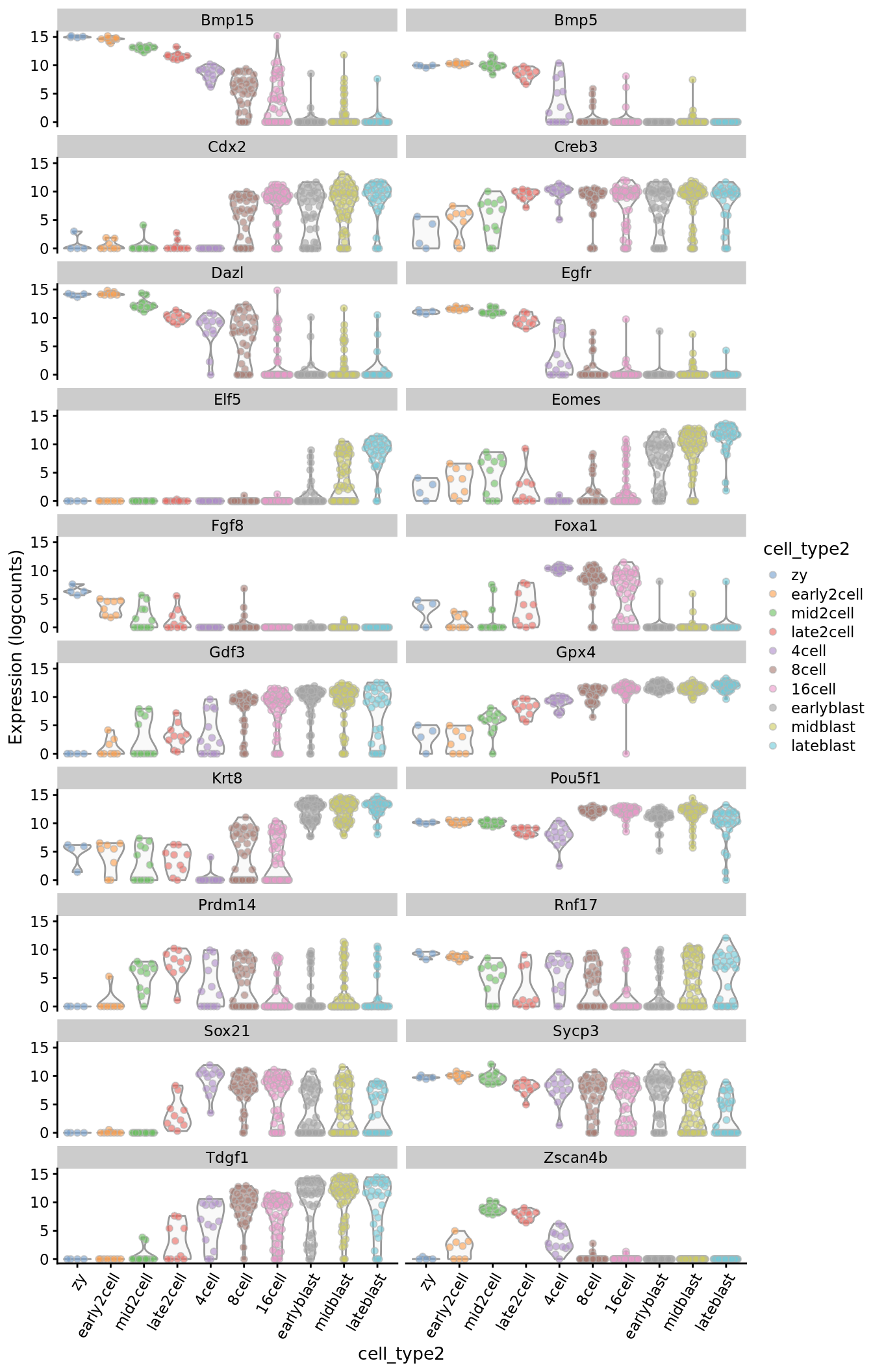
In order to fit the pseudotimes wesimply call ouija, passing in the expected response types. Note that if no response types are provided then they are all assumed to be switch-like by default, which we will do here. The input to Ouija can be a cell-by-gene matrix of non-negative expression values, or an ExpressionSet object, or, happily, by selecting the logcounts values from a SingleCellExperiment object.
We can apply prior information about whether genes are up- or down-regulated across the differentiation process, and also provide prior information about when the switch in expression or a peak in expression is likely to occur.
We can fit the Ouija model using either:
- Hamiltonian Monte Carlo (HMC) - full MCMC inference where gradient information of the log-posterior is used to “guide” the random walk through the parameter space, or
- Automatic Differentiation Variational Bayes (ADVI or simply VI) - approximate inference where the KL divergence to an approximate distribution is minimised.
In general, HMC will provide more accurate inference with approximately correct posterior variance for all parameters. However, VB is orders of magnitude quicker than HMC and while it may underestimate posterior variance, the Ouija authors suggest that anecdotally it often performs as well as HMC for discovering posterior pseudotimes.
To help the Ouija model, we provide it with prior information about the strength of switches for up- and down-regulated genes. By setting switch strength to -10 for down-regulated genes and 10 for up-regulated genes with a prior strength standard deviation of 0.5 we are telling the model that we are confident about the expected behaviour of these genes across the differentiation process.
options(mc.cores = parallel::detectCores())
response_type <- c(rep("switch", length(ouija_markers_down) +
                           length(ouija_markers_up)),
                   rep("transient", length(ouija_markers_transient)))
switch_strengths <- c(rep(-10, length(ouija_markers_down)),
                      rep(10, length(ouija_markers_up)))
switch_strength_sd <- c(rep(0.5, length(ouija_markers_down)),
                      rep(0.5, length(ouija_markers_up)))
garbage <- capture.output(
    oui_vb <- ouija(deng_SCE[ouija_markers,],
                    single_cell_experiment_assay = "logcounts",
                    response_type = response_type,
                    switch_strengths = switch_strengths,
                    switch_strength_sd = switch_strength_sd,
                    inference_type = "vb")
)

print(oui_vb)
## A Ouija fit with 268 cells and 20 marker genes
## Inference type: Variational Bayes
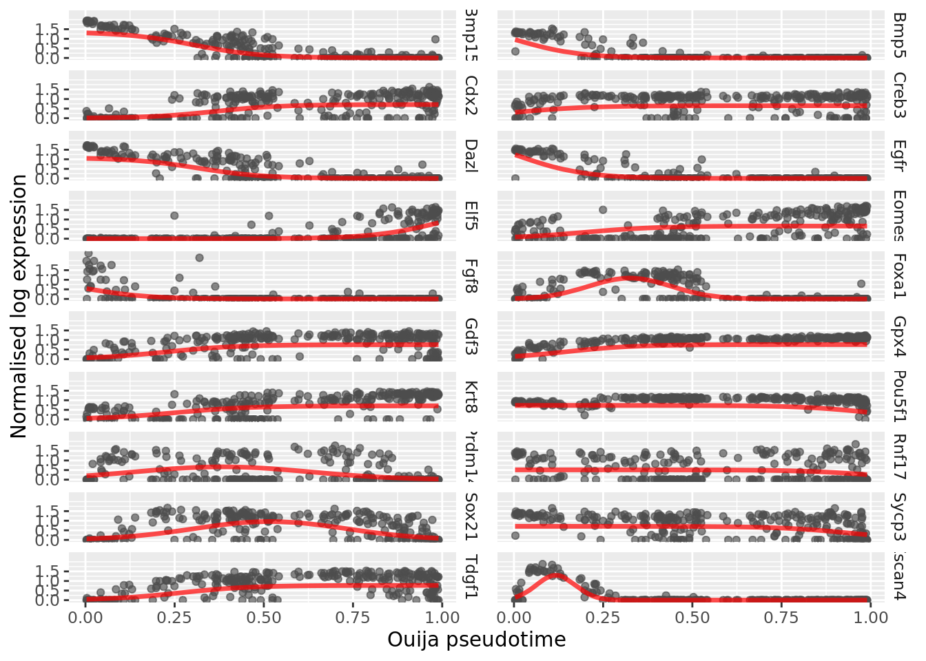
## (Gene behaviour) Switch/transient: 16 / 4We can plot the gene expression over pseudotime along with the maximum a posteriori (MAP) estimates of the mean function (the sigmoid or Gaussian transient function) using the plot_expression function.
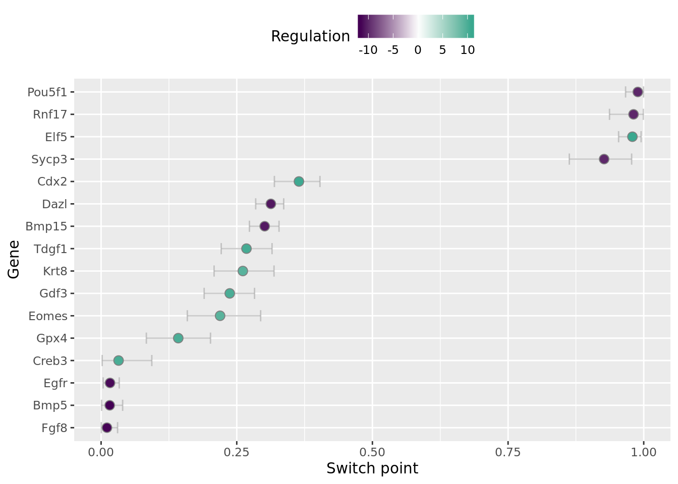
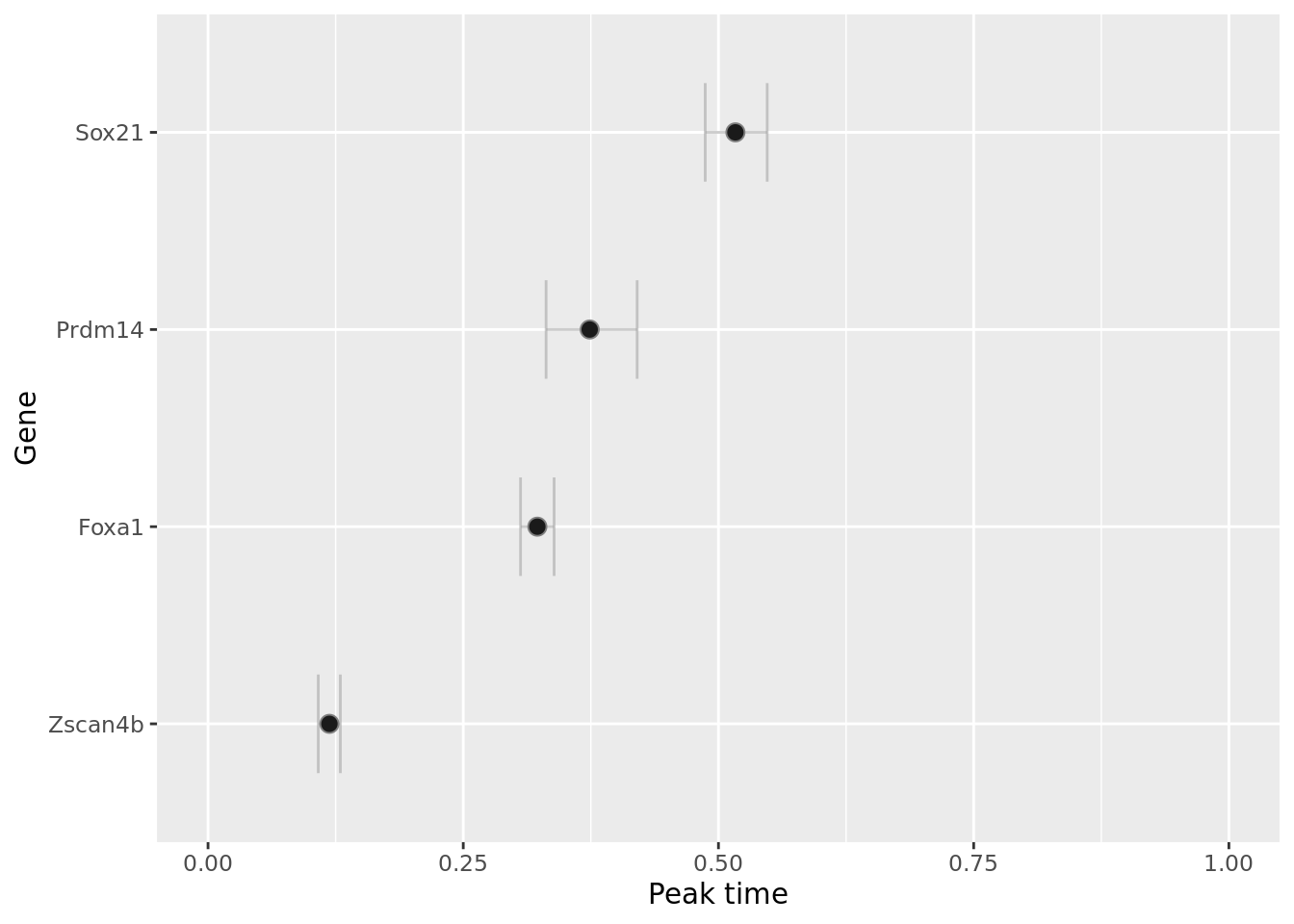
We can also visualise when in the trajectory gene regulation behaviour occurs, either in the form of the switch time or the peak time (for switch-like or transient genes) using the plot_switch_times and plot_transient_times functions:
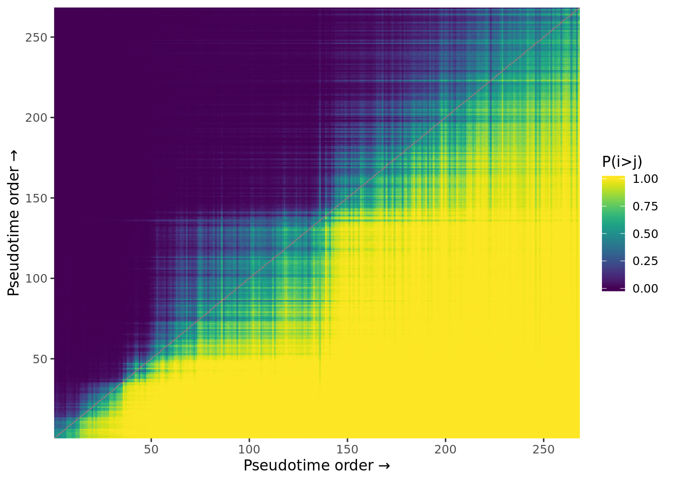
Identify metastable states using consistency matrices.
map_pst <- map_pseudotime(oui_vb)
ouija_pseudotime <- data.frame(map_pst, cell_classifications)

ggplot(ouija_pseudotime, aes(x = map_pst, y = cell_classifications)) +
  geom_point() +
  xlab("MAP pseudotime") +
  ylab("Cell classification")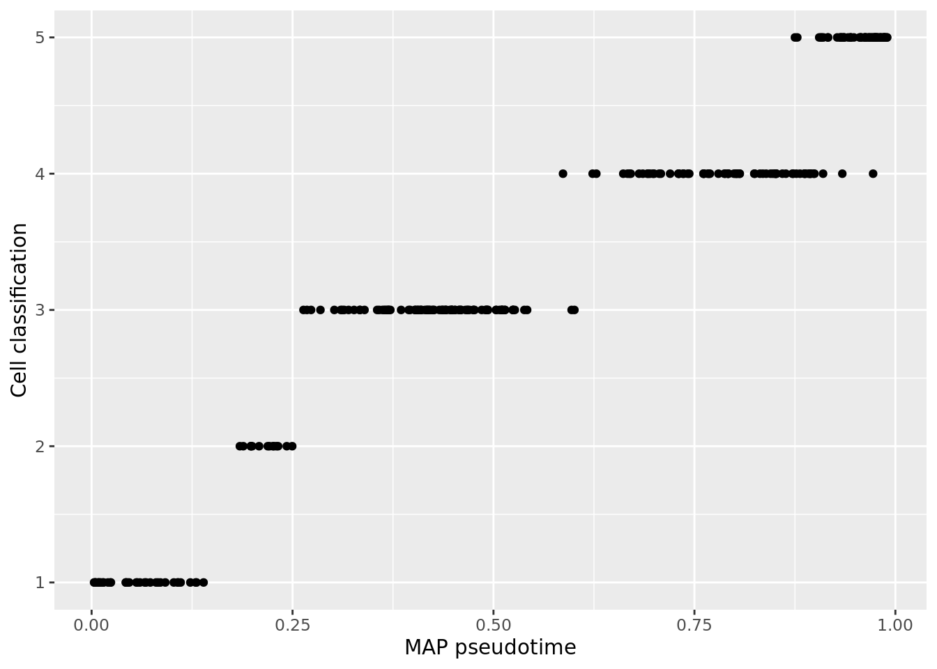
deng_SCE$pseudotime_ouija <- ouija_pseudotime$map_pst
deng_SCE$ouija_cell_class <- ouija_pseudotime$cell_classifications

ggplot(as.data.frame(colData(deng_SCE)),
       aes(x = pseudotime_ouija,
           y = cell_type2, colour = cell_type2)) +
    geom_quasirandom(groupOnX = FALSE) +
    scale_color_manual(values = my_color) + theme_classic() +
    xlab("Ouija pseudotime") +
    ylab("Timepoint") +
    theme_classic()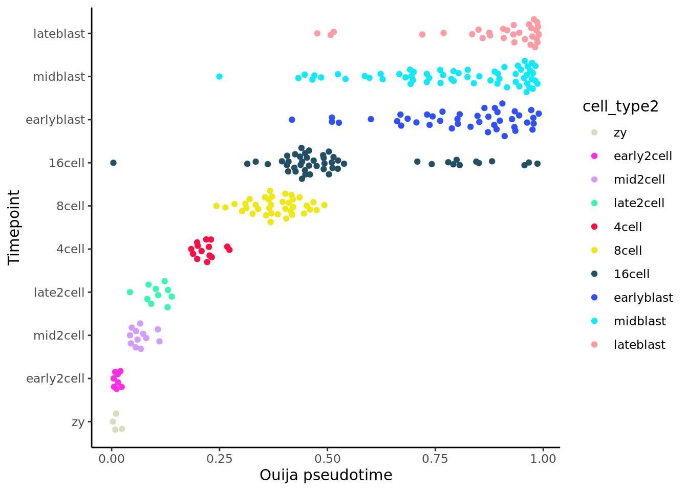
Ouija does quite well in the ordering of the cells here, although it can be sensitive to the choice of marker genes and prior information supplied. How do the results change if you select different marker genes or change the priors?
Ouija identifies four metastable states here, which we might annotate as “zygote/2cell”, “4/8/16 cell”, “blast1” and “blast2”.
ggplot(as.data.frame(colData(deng_SCE)),
       aes(x = as.factor(ouija_cell_class),
           y = pseudotime_ouija, colour = cell_type2)) +
    geom_boxplot() +
    coord_flip() +
    scale_color_manual(values = my_color) + theme_classic() +
    xlab("Ouija cell classification") +
    ylab("Ouija pseudotime") +
    theme_classic()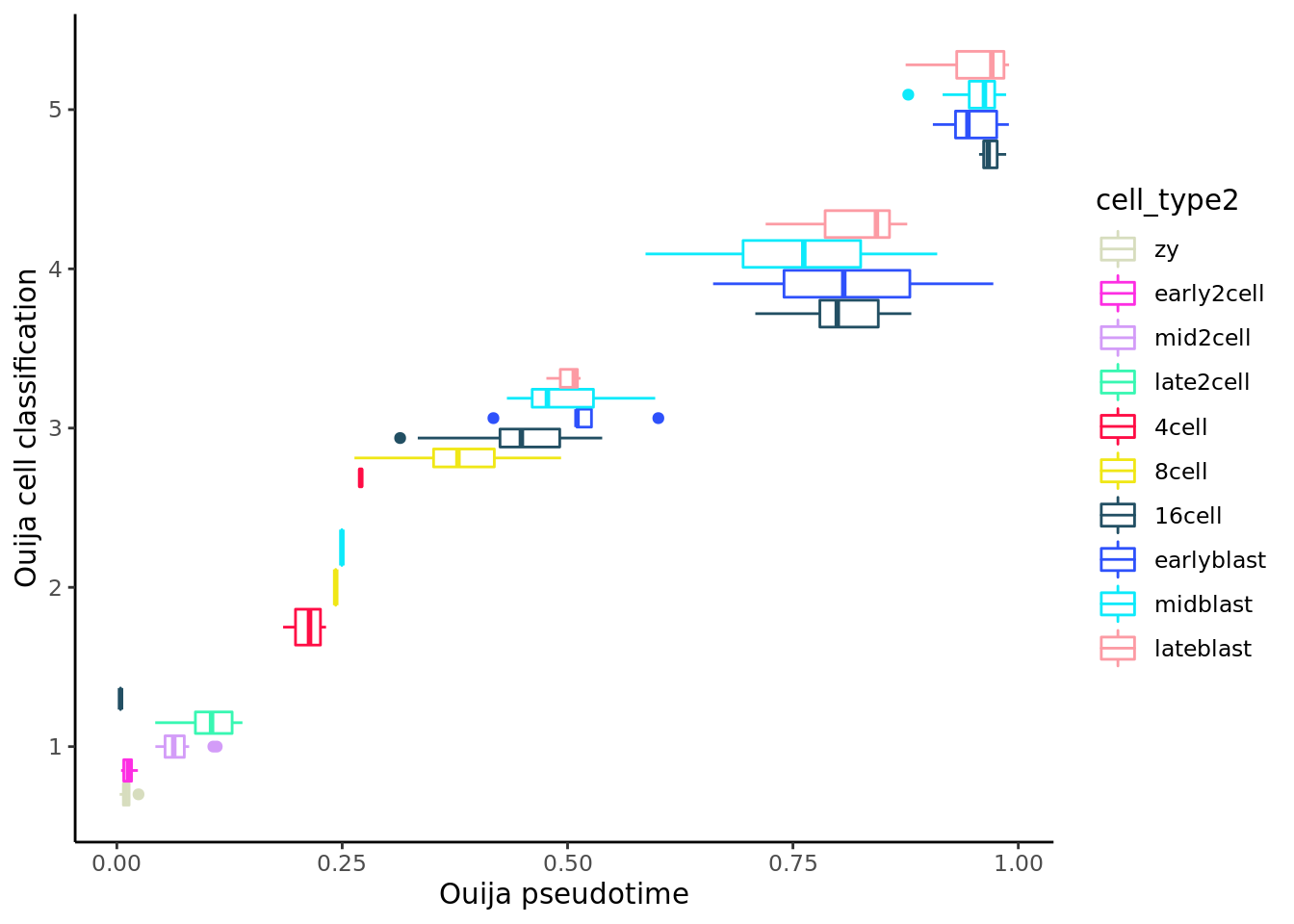
A common analysis is to work out the regulation orderings of genes. For example, is gene A upregulated before gene B? Does gene C peak before the downregulation of gene D? Ouija answers these questions in terms of a Bayesian hypothesis test of whether the difference in regulation timing (either switch time or peak time) is significantly different to 0. This is collated using the gene_regulation function.
## # A tibble: 6 x 7
## # Groups:   label, gene_A [6]
##   label         gene_A gene_B mean_difference lower_95 upper_95 significant
##   <chr>         <chr>  <chr>            <dbl>    <dbl>    <dbl> <lgl>
## 1 Bmp15 - Cdx2  Bmp15  Cdx2           -0.0631 -0.109    -0.0133 TRUE
## 2 Bmp15 - Creb3 Bmp15  Creb3           0.269   0.201     0.321  TRUE
## 3 Bmp15 - Elf5  Bmp15  Elf5           -0.678  -0.718    -0.644  TRUE
## 4 Bmp15 - Eomes Bmp15  Eomes           0.0822  0.00272   0.156  TRUE
## 5 Bmp15 - Foxa1 Bmp15  Foxa1          -0.0211 -0.0508    0.0120 FALSE
## 6 Bmp15 - Gdf3  Bmp15  Gdf3            0.0644  0.0163    0.126  TRUE
What conclusions can you draw from the gene regulation output from Ouija?
If you have time, you might try the HMC inference method and see if that changes the Ouija results in any way.
11.6 Comparison of the methods
How do the trajectories inferred by TSCAN, Monocle, Diffusion Map, SLICER and Ouija compare?
TSCAN and Diffusion Map methods get the trajectory the “wrong way round”, so we’ll adjust that for these comparisons.
df_pseudotime <- as.data.frame(
    colData(deng_SCE)[, grep("pseudotime", colnames(colData(deng_SCE)))]
)
colnames(df_pseudotime) <- gsub("pseudotime_", "",
                                colnames(df_pseudotime))
df_pseudotime$PC1 <- reducedDim(deng_SCE,"PCA")[,1]
df_pseudotime$order_tscan <- -df_pseudotime$order_tscan
#df_pseudotime$diffusionmap <- df_pseudotime$diffusionmap
df_pseudotime$slingshot1 <- colData(deng_SCE)$slingPseudotime_1

corrplot.mixed(cor(df_pseudotime, use = "na.or.complete"),
               order = "hclust", tl.col = "black",
               main = "Correlation matrix for pseudotime results",
               mar = c(0, 0, 3.1, 0))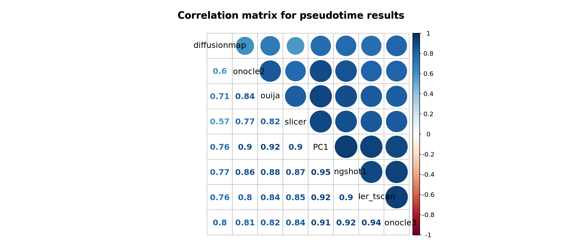
We see here that Ouija, TSCAN and SLICER all give trajectories that are similar and strongly correlated with PC1. Diffusion Map is less strongly correlated with these methods, and Monocle gives very different results.
11.7 Expression of genes through time
Each package also enables the visualization of expression through pseudotime. Following individual genes is very helpful for identifying genes that play an important role in the differentiation process. We illustrate the procedure using the Nanog gene.
We have added the pseudotime values computed with all methods here to
the colData slot of an SCE object. Having done that, the full
plotting capabilities of the scater package can be used to
investigate relationships between gene expression, cell populations
and pseudotime. This is particularly useful for the packages such as
SLICER that do not provide plotting functions.
Principal components
deng_SCE$PC1 <- reducedDim(deng_SCE,"PCA")[,1]
plotExpression(deng_SCE, "Nanog", x = "PC1",
               colour_by = "cell_type2", show_violin = FALSE,
               show_smooth = TRUE)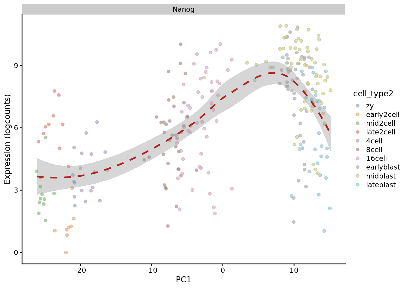
TSCAN
plotExpression(deng_SCE, "Nanog", x = "pseudotime_order_tscan",
               colour_by = "cell_type2", show_violin = FALSE,
               show_smooth = TRUE)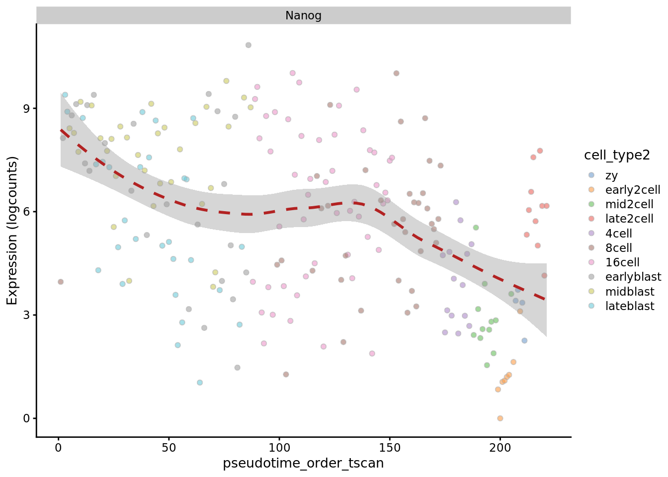
Monocle
plotExpression(deng_SCE, "Nanog", x = "pseudotime_monocle2",
               colour_by = "cell_type2", show_violin = FALSE,
               show_smooth = TRUE)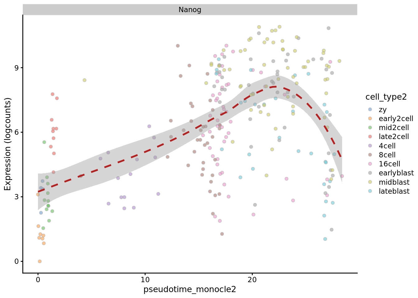
Diffusion Map
plotExpression(deng_SCE, "Nanog", x = "pseudotime_diffusionmap",
               colour_by = "cell_type2", show_violin = FALSE,
               show_smooth = TRUE)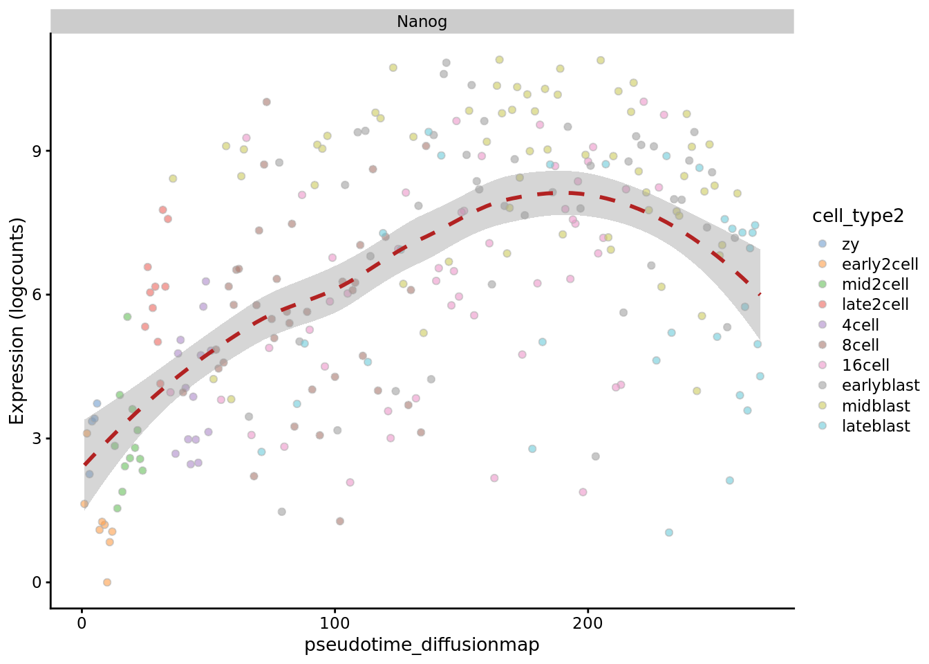
SLICER
plotExpression(deng_SCE, "Nanog", x = "pseudotime_slicer",
               colour_by = "cell_type2", show_violin = FALSE,
               show_smooth = TRUE)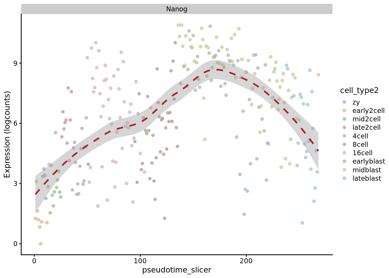
Ouija
plotExpression(deng_SCE, "Nanog", x = "pseudotime_ouija",
               colour_by = "cell_type2", show_violin = FALSE,
               show_smooth = TRUE)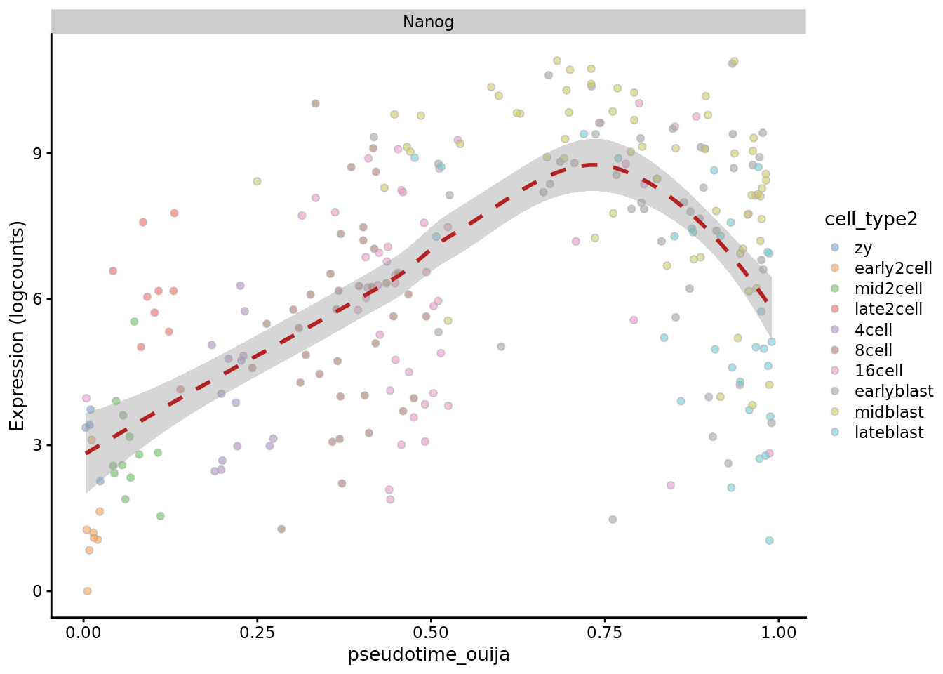
Q: How many of these methods outperform the naive approach of using the first principal component to represent pseudotime for these data?
Exercise 7: Repeat the exercise using a subset of the genes, e.g. the set of highly variable genes that can be obtained using one of the methods discussed in the Feature Selection chapter.
11.7.1 dynverse
https://dynverse.org/users/2-quick_start/
library(dyno)
library(tidyverse)

# Reproduces the guidelines as created in the shiny app
answers <- dynguidelines::answer_questions(
  multiple_disconnected = FALSE,
  expect_topology = TRUE,
  expected_topology = "linear",
  n_cells = 3000,
  n_features = 10000,
  memory = "100GB",
  docker = FALSE
)
guidelines <- dynguidelines::guidelines(answers = answers)
guidelines


deng_dataset <- wrap_expression(
  counts = counts(deng_SCE),
  expression = assay(deng_SCE,"logcounts")

)
model <- infer_trajectory(deng_dataset, first(guidelines$methods_selected))
## Loading required namespace: hdf5r

model <- model %>% add_dimred(dyndimred::dimred_mds,
                              expression_source = deng_dataset$expression)
plot_dimred(
  model,
  expression_source = deng_dataset$expression,
  grouping = deng_SCE$cell_type2
)
11.7.2 sessionInfo()
## R version 3.6.0 (2019-04-26)
## Platform: x86_64-pc-linux-gnu (64-bit)
## Running under: Ubuntu 18.04.3 LTS
##
## Matrix products: default
## BLAS:   /usr/lib/x86_64-linux-gnu/blas/libblas.so.3.7.1
## LAPACK: /usr/lib/x86_64-linux-gnu/lapack/liblapack.so.3.7.1
##
## locale:
##  [1] LC_CTYPE=en_AU.UTF-8       LC_NUMERIC=C
##  [3] LC_TIME=en_AU.UTF-8        LC_COLLATE=en_AU.UTF-8
##  [5] LC_MONETARY=en_AU.UTF-8    LC_MESSAGES=en_AU.UTF-8
##  [7] LC_PAPER=en_AU.UTF-8       LC_NAME=C
##  [9] LC_ADDRESS=C               LC_TELEPHONE=C
## [11] LC_MEASUREMENT=en_AU.UTF-8 LC_IDENTIFICATION=C
##
## attached base packages:
##  [1] splines   parallel  stats4    stats     graphics  grDevices utils
##  [8] datasets  methods   base
##
## other attached packages:
##  [1] rstan_2.19.2                StanHeaders_2.19.0
##  [3] lle_1.1                     snowfall_1.84-6.1
##  [5] snow_0.4-3                  MASS_7.3-51.1
##  [7] scatterplot3d_0.3-41        monocle3_0.2.0
##  [9] gam_1.16.1                  foreach_1.4.7
## [11] ouija_0.99.0                Rcpp_1.0.2
## [13] SLICER_0.2.0                slingshot_1.2.0
## [15] princurve_2.1.4             Polychrome_1.2.3
## [17] corrplot_0.84               ggbeeswarm_0.6.0
## [19] ggthemes_4.2.0              scater_1.12.2
## [21] destiny_2.14.0              monocle_2.12.0
## [23] DDRTree_0.1.5               irlba_2.3.3
## [25] VGAM_1.1-1                  ggplot2_3.2.1
## [27] Matrix_1.2-17               M3Drop_1.10.0
## [29] numDeriv_2016.8-1.1         TSCAN_1.22.0
## [31] SingleCellExperiment_1.6.0  SummarizedExperiment_1.14.1
## [33] DelayedArray_0.10.0         BiocParallel_1.18.1
## [35] matrixStats_0.55.0          Biobase_2.44.0
## [37] GenomicRanges_1.36.1        GenomeInfoDb_1.20.0
## [39] IRanges_2.18.3              S4Vectors_0.22.1
## [41] BiocGenerics_0.30.0
##
## loaded via a namespace (and not attached):
##   [1] rgl_0.100.30             rsvd_1.0.2
##   [3] vcd_1.4-4                Hmisc_4.2-0
##   [5] zinbwave_1.6.0           corpcor_1.6.9
##   [7] ps_1.3.0                 class_7.3-15
##   [9] lmtest_0.9-37            glmnet_2.0-18
##  [11] crayon_1.3.4             laeken_0.5.0
##  [13] nlme_3.1-139             backports_1.1.4
##  [15] qlcMatrix_0.9.7          rlang_0.4.0
##  [17] XVector_0.24.0           readxl_1.3.1
##  [19] callr_3.3.2              limma_3.40.6
##  [21] phylobase_0.8.6          smoother_1.1
##  [23] manipulateWidget_0.10.0  bit64_0.9-7
##  [25] loo_2.1.0                glue_1.3.1
##  [27] pheatmap_1.0.12          rngtools_1.4
##  [29] splancs_2.01-40          processx_3.4.1
##  [31] vipor_0.4.5              AnnotationDbi_1.46.1
##  [33] haven_2.1.1              tidyselect_0.2.5
##  [35] rio_0.5.16               XML_3.98-1.20
##  [37] tidyr_1.0.0              zoo_1.8-6
##  [39] xtable_1.8-4             magrittr_1.5
##  [41] evaluate_0.14            bibtex_0.4.2
##  [43] cli_1.1.0                zlibbioc_1.30.0
##  [45] rstudioapi_0.10          miniUI_0.1.1.1
##  [47] sp_1.3-1                 rpart_4.1-15
##  [49] locfdr_1.1-8             RcppEigen_0.3.3.5.0
##  [51] shiny_1.3.2              BiocSingular_1.0.0
##  [53] xfun_0.9                 leidenbase_0.1.0
##  [55] inline_0.3.15            pkgbuild_1.0.5
##  [57] cluster_2.1.0            caTools_1.17.1.2
##  [59] sgeostat_1.0-27          tibble_2.1.3
##  [61] ggrepel_0.8.1            ape_5.3
##  [63] stabledist_0.7-1         zeallot_0.1.0
##  [65] withr_2.1.2              bitops_1.0-6
##  [67] slam_0.1-45              ranger_0.11.2
##  [69] plyr_1.8.4               cellranger_1.1.0
##  [71] pcaPP_1.9-73             sparsesvd_0.2
##  [73] coda_0.19-3              e1071_1.7-2
##  [75] RcppParallel_4.4.3       pillar_1.4.2
##  [77] gplots_3.0.1.1           reldist_1.6-6
##  [79] kernlab_0.9-27           TTR_0.23-5
##  [81] ellipsis_0.3.0           tripack_1.3-8
##  [83] DelayedMatrixStats_1.6.1 xts_0.11-2
##  [85] vctrs_0.2.0              NMF_0.21.0
##  [87] tools_3.6.0              foreign_0.8-70
##  [89] rncl_0.8.3               beeswarm_0.2.3
##  [91] munsell_0.5.0            proxy_0.4-23
##  [93] HSMMSingleCell_1.4.0     compiler_3.6.0
##  [95] abind_1.4-5              httpuv_1.5.2
##  [97] pkgmaker_0.27            GenomeInfoDbData_1.2.1
##  [99] gridExtra_2.3            edgeR_3.26.8
## [101] lattice_0.20-38          deldir_0.1-23
## [103] utf8_1.1.4               later_0.8.0
## [105] dplyr_0.8.3              jsonlite_1.6
## [107] scales_1.0.0             docopt_0.6.1
## [109] carData_3.0-2            genefilter_1.66.0
## [111] lazyeval_0.2.2           promises_1.0.1
## [113] spatstat_1.61-0          car_3.0-3
## [115] doParallel_1.0.15        latticeExtra_0.6-28
## [117] R.utils_2.9.0            goftest_1.1-1
## [119] spatstat.utils_1.13-0    checkmate_1.9.4
## [121] cowplot_1.0.0            rmarkdown_1.15
## [123] openxlsx_4.1.0.1         statmod_1.4.32
## [125] webshot_0.5.1            Rtsne_0.15
## [127] forcats_0.4.0            copula_0.999-19.1
## [129] softImpute_1.4           uwot_0.1.4
## [131] igraph_1.2.4.1           HDF5Array_1.12.2
## [133] survival_2.43-3          yaml_2.2.0
## [135] htmltools_0.3.6          memoise_1.1.0
## [137] locfit_1.5-9.1           viridisLite_0.3.0
## [139] digest_0.6.21            assertthat_0.2.1
## [141] mime_0.7                 densityClust_0.3
## [143] registry_0.5-1           RSQLite_2.1.2
## [145] data.table_1.12.2        blob_1.2.0
## [147] R.oo_1.22.0              RNeXML_2.3.0
## [149] labeling_0.3             fastICA_1.2-2
## [151] Formula_1.2-3            Rhdf5lib_1.6.1
## [153] RCurl_1.95-4.12          hms_0.5.1
## [155] rhdf5_2.28.0             colorspace_1.4-1
## [157] base64enc_0.1-3          nnet_7.3-12
## [159] ADGofTest_0.3            mclust_5.4.5
## [161] bookdown_0.13            RANN_2.6.1
## [163] mvtnorm_1.0-11           fansi_0.4.0
## [165] pspline_1.0-18           VIM_4.8.0
## [167] R6_2.4.0                 grid_3.6.0
## [169] lifecycle_0.1.0          acepack_1.4.1
## [171] zip_2.0.4                curl_4.2
## [173] gdata_2.18.0             robustbase_0.93-5
## [175] howmany_0.3-1            RcppAnnoy_0.0.13
## [177] RColorBrewer_1.1-2       MCMCglmm_2.29
## [179] iterators_1.0.12         alphahull_2.2
## [181] stringr_1.4.0            htmlwidgets_1.3
## [183] polyclip_1.10-0          purrr_0.3.2
## [185] crosstalk_1.0.0          mgcv_1.8-28
## [187] tensorA_0.36.1           htmlTable_1.13.2
## [189] clusterExperiment_2.4.4  codetools_0.2-16
## [191] FNN_1.1.3                gtools_3.8.1
## [193] prettyunits_1.0.2        gridBase_0.4-7
## [195] RSpectra_0.15-0          R.methodsS3_1.7.1
## [197] gtable_0.3.0             DBI_1.0.0
## [199] highr_0.8                tensor_1.5
## [201] httr_1.4.1               KernSmooth_2.23-15
## [203] stringi_1.4.3            progress_1.2.2
## [205] reshape2_1.4.3           uuid_0.1-2
## [207] cubature_2.0.3           annotate_1.62.0
## [209] viridis_0.5.1            xml2_1.2.2
## [211] combinat_0.0-8           bbmle_1.0.20
## [213] boot_1.3-20              BiocNeighbors_1.2.0
## [215] ade4_1.7-13              DEoptimR_1.0-8
## [217] bit_1.1-14               spatstat.data_1.4-0
## [219] pkgconfig_2.0.3          gsl_2.1-6
## [221] knitr_1.25
References
Angerer, Philipp, Laleh Haghverdi, Maren Büttner, Fabian J Theis, Carsten Marr, and Florian Buettner. 2016. “Destiny: Diffusion Maps for Large-Scale Single-Cell Data in R.” Bioinformatics 32 (8): 1241–3.
Cao, Junyue, Malte Spielmann, Xiaojie Qiu, Xingfan Huang, Daniel M Ibrahim, Andrew J Hill, Fan Zhang, et al. 2019. “The Single-Cell Transcriptional Landscape of Mammalian Organogenesis.” Nature 566 (7745): 496–502.
Coifman, Ronald R, and Stéphane Lafon. 2006. “Diffusion Maps.” Appl. Comput. Harmon. Anal. 21 (1): 5–30.
Deng, Q., D. Ramskold, B. Reinius, and R. Sandberg. 2014. “Single-Cell RNA-Seq Reveals Dynamic, Random Monoallelic Gene Expression in Mammalian Cells.” Science 343 (6167). American Association for the Advancement of Science (AAAS): 193–96. https://doi.org/10.1126/science.1245316.
Hastie, Trevor, and Werner Stuetzle. 1989. “Principal Curves.” AT&T Bell Laboratorie,Murray Hill; Journal of the American Statistical Association.
Ji, Zhicheng, and Hongkai Ji. 2019. TSCAN: TSCAN: Tools for Single-Cell Analysis.
Qiu, Xiaojie, Qi Mao, Ying Tang, Li Wang, Raghav Chawla, Hannah A Pliner, and Cole Trapnell. 2017. “Reversed Graph Embedding Resolves Complex Single-Cell Trajectories.” Nat. Methods 14 (10): 979–82.
Saelens, Wouter, Robrecht Cannoodt, Helena Todorov, and Yvan Saeys. 2019. “A Comparison of Single-Cell Trajectory Inference Methods.” Nature Biotechnology 37 (5). Nature Publishing Group: 547.
Street, Kelly, Davide Risso, Russell B Fletcher, Diya Das, John Ngai, Nir Yosef, Elizabeth Purdom, and Sandrine Dudoit. 2018. “Slingshot: Cell Lineage and Pseudotime Inference for Single-Cell Transcriptomics.” BMC Genomics 19 (1): 477.
Trapnell, Cole, Davide Cacchiarelli, Jonna Grimsby, Prapti Pokharel, Shuqiang Li, Michael Morse, Niall J Lennon, Kenneth J Livak, Tarjei S Mikkelsen, and John L Rinn. 2014. “The Dynamics and Regulators of Cell Fate Decisions Are Revealed by Pseudotemporal Ordering of Single Cells.” Nat. Biotechnol. 32 (4): 381–86.
Welch, Joshua D., Alexander J. Hartemink, and Jan F. Prins. 2016. “SLICER: Inferring Branched, Nonlinear Cellular Trajectories from Single Cell RNA-Seq Data.” Genome Biol 17 (1). Springer Nature. https://doi.org/10.1186/s13059-016-0975-3.