14 Comparing and combining scRNA-seq datasets
14.1 Introduction
As more and more scRNA-seq datasets become available, carrying merged_seurat comparisons between them is key. There are two main approaches to comparing scRNASeq datasets. The first approach is “label-centric” which is focused on trying to identify equivalent cell-types/states across datasets by comparing individual cells or groups of cells. The other approach is “cross-dataset normalization” which attempts to computationally remove experiment-specific technical/biological effects so that data from multiple experiments can be combined and jointly analyzed.
The label-centric approach can be used with dataset with high-confidence cell-annotations, e.g. the Human Cell Atlas (HCA) (Regev et al. 2017) or the Tabula Muris (???) once they are completed, to project cells or clusters from a new sample onto this reference to consider tissue composition and/or identify cells with novel/unknown identity. Conceptually, such projections are similar to the popular BLAST method (Altschul et al. 1990), which makes it possible to quickly find the closest match in a database for a newly identified nucleotide or amino acid sequence. The label-centric approach can also be used to compare datasets of similar biological origin collected by different labs to ensure that the annotation and the analysis is consistent.
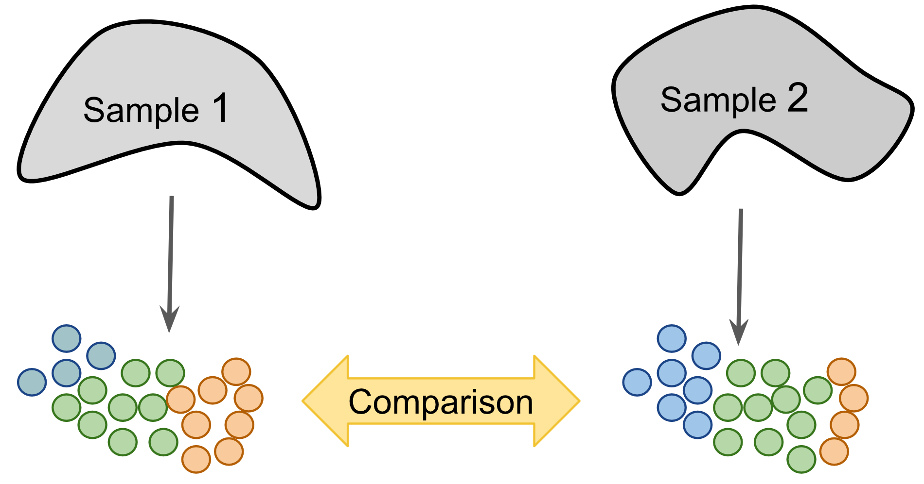
Figure 2.4: Label-centric dataset comparison can be used to compare the annotations of two different samples.
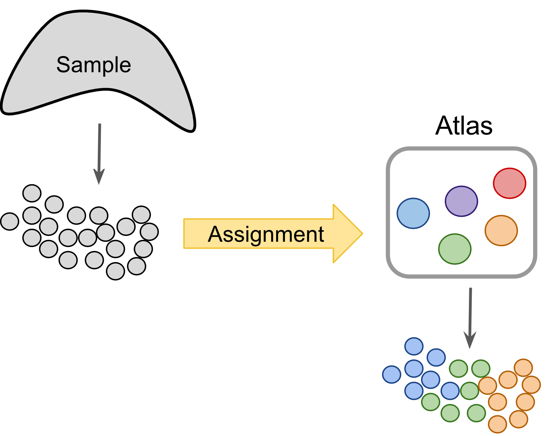
Figure 2.5: Label-centric dataset comparison can project cells from a new experiment onto an annotated reference.
The cross-dataset normalization approach can also be used to compare datasets of similar biological origin, unlike the label-centric approach it enables the join analysis of multiple datasets to facilitate the identification of rare cell-types which may to too sparsely sampled in each individual dataset to be reliably detected. However, cross-dataset normalization is not applicable to very large and diverse references since it assumes a significant portion of the biological variablility in each of the datasets overlaps with others.
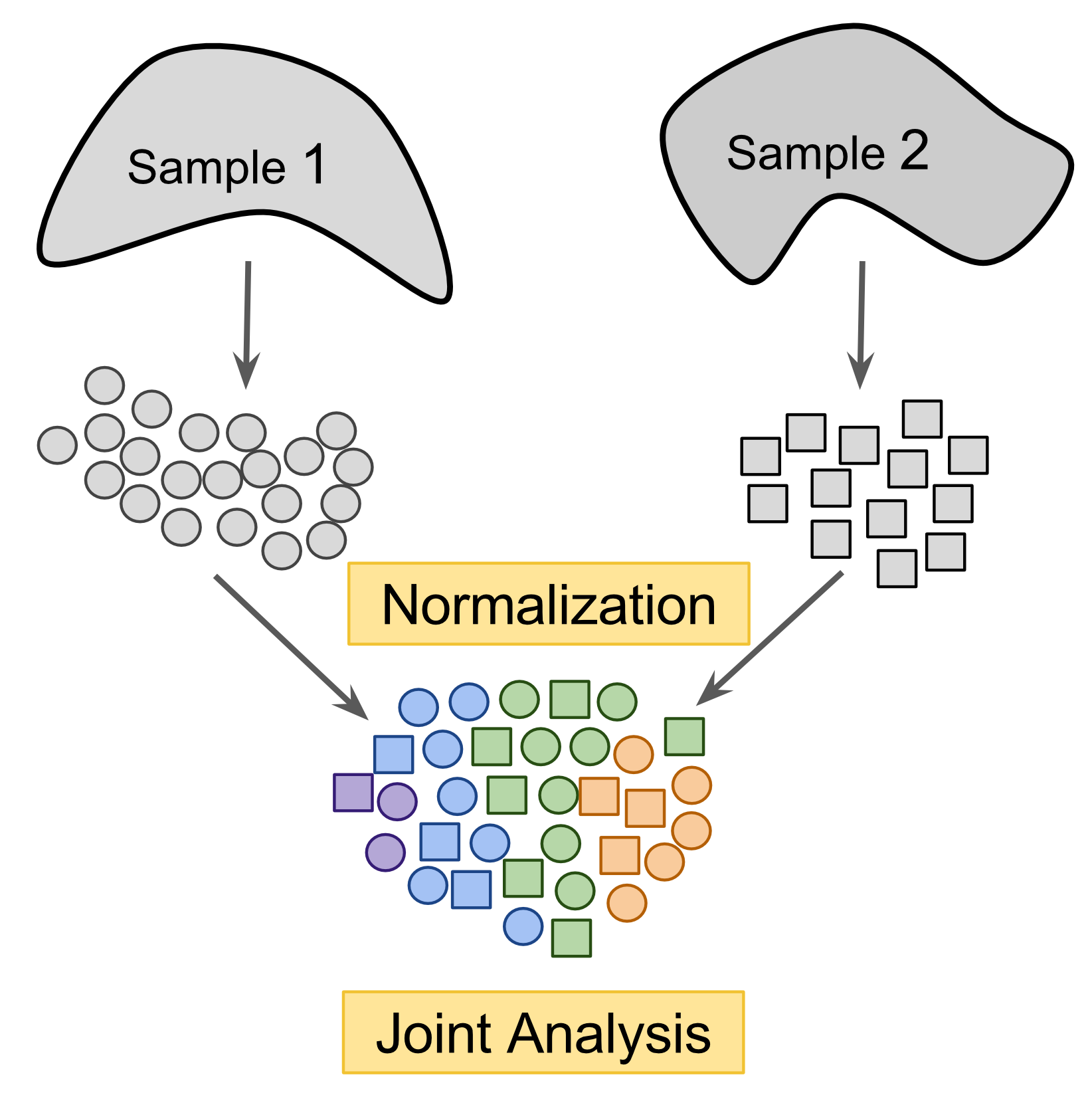
Figure 2.6: Cross-dataset normalization enables joint-analysis of 2+ scRNASeq datasets.
14.2 Datasets
We will running these methods on two human pancreas datasets: (Muraro et al. 2016) and (Segerstolpe et al. 2016). Since the pancreas has been widely studied, these datasets are well annotated.
muraro <- readRDS("data/pancreas/muraro.rds")
segerstolpe <- readRDS("data/pancreas/segerstolpe.rds")This data has already been formatted for scmap. Cell type labels must be stored
in the cell_type1 column of the colData slots, and gene ids that are
consistent across both datasets must be stored in the feature_symbol column of
the rowData slots.
First, lets check our gene-ids match across both datasets:
## [1] 0.9599519## [1] 0.719334Here we can see that 96% of the genes present in muraro match genes in segerstople and 72% of genes in segerstolpe are match genes in muraro. This is as expected because the segerstolpe dataset was more deeply sequenced than the muraro dataset. However, it highlights some of the difficulties in comparing scRNASeq datasets.
We can confirm this by checking the overall size of these two datasets.
## [1] 19127 2126## [1] 25525 3514In addition, we can check the cell-type annotations for each of these dataset using the command below:
## acinar alpha beta delta ductal endothelial
## 219 812 448 193 245 21
## epsilon gamma mesenchymal unclear
## 3 101 80 4## acinar alpha beta
## 185 886 270
## co-expression delta ductal
## 39 114 386
## endothelial epsilon gamma
## 16 7 197
## mast MHC class II not applicable
## 7 5 1305
## PSC unclassified unclassified endocrine
## 54 2 41Here we can see that even though both datasets considered the same biological
tissue, they have been annotated with slightly different sets of cell-types. If
you are familiar with pancreas biology you might recognize that the pancreatic
stellate cells (PSCs) in segerstolpe are a type of mesenchymal stem cell which
would fall under the “mesenchymal” type in muraro. However, it isn’t clear
whether these two annotations should be considered synonymous or not. We can use
label-centric comparison methods to determine if these two cell-type annotations
are indeed equivalent.
Alternatively, we might be interested in understanding the function of those cells that were “unclassified endocrine” or were deemed too poor quality (“not applicable”) for the original clustering in each dataset by leveraging in formation across datasets. Either we could attempt to infer which of the existing annotations they most likely belong to using label-centric approaches or we could try to uncover a novel cell-type among them (or a sub-type within the existing annotations) using cross-dataset normalization.
To simplify our demonstration analyses we will remove the small classes of unassigned cells, and the poor quality cells. We will retain the “unclassified endocrine” to see if any of these methods can elucidate what cell-type they belong to.
14.3 Projecting cells onto annotated cell-types (scmap)
Martin Hemberg and colleagues recently developed scmap (Kiselev and Hemberg 2017)—a
method for projecting cells from a scRNA-seq experiment onto the cell-types
identified in other experiments. Additionally, a cloud version of scmap can be
run for free, without restrictions, from
http://www.hemberg-lab.cloud/scmap.
14.3.0.1 Feature Selection
Once we have a SingleCellExperiment object we can run scmap. First we have
to build the “index” of our reference clusters. Since we want to know whether
PSCs and mesenchymal cells are synonymous we will project each dataset to the
other so we will build an index for each dataset. This requires first selecting
the most informative features for the reference dataset.
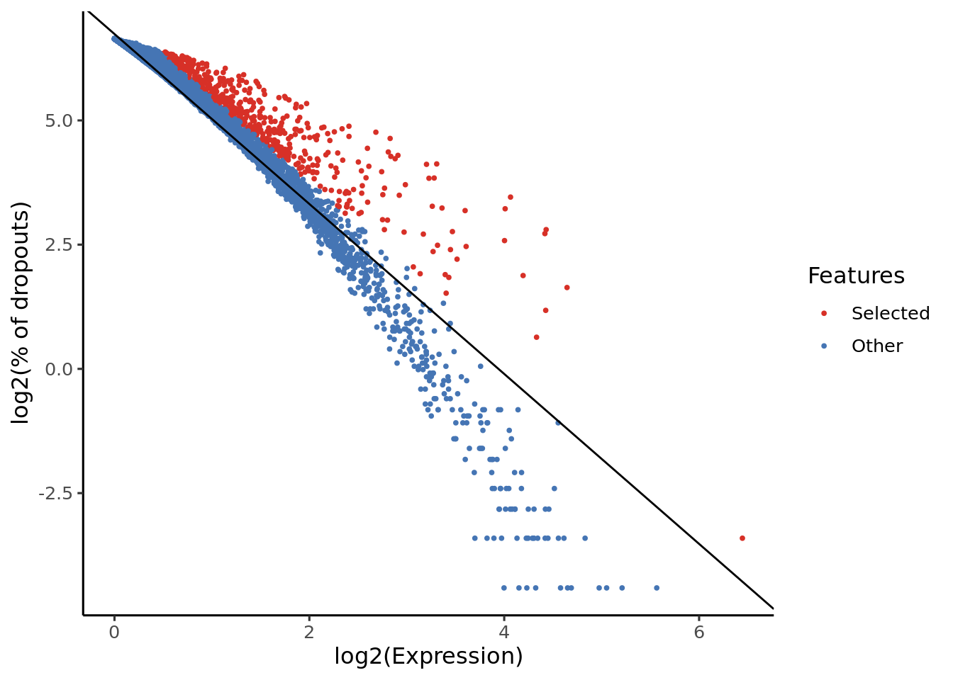
Genes highlighted with the red colour will be used in the futher analysis (projection).
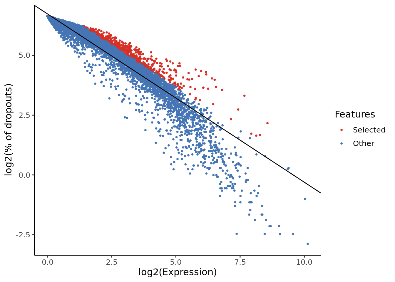
From the y-axis of these plots we can see that scmap uses a dropmerged_seurat-based feature selection method.
Now calculate the cell-type index:
We can also visualize the index:
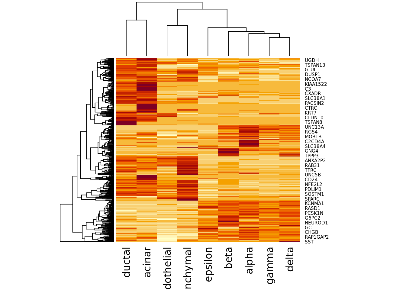
You may want to adjust your features using the setFeatures function if
features are too heavily concentrated in only a few cell-types. In this case the
dropout-based features look good so we will just them.
Exercise Using the rowData of each dataset how many genes were selected as features in both datasets? What does this tell you about these datasets?
Answer
14.3.1 Projecting
scmap computes the distance from each cell to each cell-type in the reference index, then applies an empirically derived threshold to determine which cells are assigned to the closest reference cell-type and which are unassigned. To account for differences in sequencing depth distance is calculated using the spearman correlation and cosine distance and only cells with a consistent assignment with both distances are returned as assigned.
We will project the segerstolpe dataset to muraro dataset:
seger_to_muraro <- scmapCluster(
projection = segerstolpe,
index_list = list(
muraro = metadata(muraro)$scmap_cluster_index
)
)and muraro onto segerstolpe
muraro_to_seger <- scmapCluster(
projection = muraro,
index_list = list(
seger = metadata(segerstolpe)$scmap_cluster_index
)
)Note that in each case we are projecting to a single dataset but that this could be extended to any number of datasets for which we have computed indices.
Now lets compare the original cell-type labels with the projected labels:
##
## acinar alpha beta co-expression delta ductal endothelial
## acinar 211 0 0 0 0 0 0
## alpha 1 763 0 18 0 2 0
## beta 2 1 397 7 2 2 0
## delta 0 0 2 1 173 0 0
## ductal 7 0 0 0 0 208 0
## endothelial 0 0 0 0 0 0 15
## epsilon 0 0 0 0 0 0 0
## gamma 2 0 0 0 0 0 0
## mesenchymal 0 0 0 0 0 1 0
##
## epsilon gamma MHC class II PSC unassigned
## acinar 0 0 0 0 8
## alpha 0 2 0 0 26
## beta 0 5 1 2 29
## delta 0 0 0 0 17
## ductal 0 0 5 3 22
## endothelial 0 0 0 1 5
## epsilon 3 0 0 0 0
## gamma 0 95 0 0 4
## mesenchymal 0 0 0 77 2Here we can see that cell-types do map to their equivalents in segerstolpe, and importantly we see that all but one of the “mesenchymal” cells were assigned to the “PSC” class.
##
## acinar alpha beta delta ductal endothelial
## acinar 181 0 0 0 4 0
## alpha 0 869 1 0 0 0
## beta 0 0 260 0 0 0
## co-expression 0 7 31 0 0 0
## delta 0 0 1 111 0 0
## ductal 0 0 0 0 383 0
## endothelial 0 0 0 0 0 14
## epsilon 0 0 0 0 0 0
## gamma 0 2 0 0 0 0
## mast 0 0 0 0 0 0
## MHC class II 0 0 0 0 0 0
## PSC 0 0 1 0 0 0
## unclassified endocrine 0 0 0 0 0 0
##
## epsilon gamma mesenchymal unassigned
## acinar 0 0 0 0
## alpha 0 0 0 16
## beta 0 0 0 10
## co-expression 0 0 0 1
## delta 0 0 0 2
## ductal 0 0 0 3
## endothelial 0 0 0 2
## epsilon 6 0 0 1
## gamma 0 192 0 3
## mast 0 0 0 7
## MHC class II 0 0 0 5
## PSC 0 0 53 0
## unclassified endocrine 0 0 0 41Again we see cell-types match each other and that all but one of the “PSCs” match the “mesenchymal” cells providing strong evidence that these two annotations should be considered synonymous.
We can also visualize these tables using a Sankey diagram:
plot(getSankey(colData(muraro)$cell_type1, muraro_to_seger$scmap_cluster_labs[,1], plot_height=400))Exercise How many of the previously unclassified cells would be be able to assign to cell-types using scmap?
Answer
14.4 Cell-to-Cell mapping
scmap can also project each cell in one dataset to its approximate closest
neighbouring cell in the reference dataset. This uses a highly optimized search
algorithm allowing it to be scaled to very large references (in theory
100,000–millions of cells). However, this process is stochastic so we must fix
the random seed to ensure we can reproduce our results.
We have already performed feature selection for this dataset so we can go straight to building the index.
In this case the index is a series of clusterings of each cell using different sets of features, parameters k and M are the number of clusters and the number of features used in each of these subclusterings. New cells are assigned to the nearest cluster in each subclustering to generate unique pattern of cluster assignments. We then find the cell in the reference dataset with the same or most similar pattern of cluster assignments.
We can examine the cluster assignment patterns for the reference datasets using:
## D28.1_1 D28.1_13 D28.1_15 D28.1_17 D28.1_2
## [1,] 4 6 4 24 34
## [2,] 16 27 14 11 3
## [3,] 18 12 17 26 24
## [4,] 44 33 41 44 12
## [5,] 39 44 23 34 32To project and find the w nearest neighbours we use a similar command as before:
muraro_to_seger <- scmapCell(
projection = muraro,
index_list = list(
seger = metadata(segerstolpe)$scmap_cell_index
),
w = 5
)We can again look at the results:
## D28.1_1 D28.1_13 D28.1_15 D28.1_17 D28.1_2
## [1,] 1448 1381 1125 1834 1553
## [2,] 1731 855 1081 1731 1437
## [3,] 1229 2113 2104 1790 1890
## [4,] 2015 1833 1153 1882 1593
## [5,] 1159 1854 1731 1202 1078This shows the column number of the 5 nearest neighbours in segerstolpe to each of the cells in muraro. We could then calculate a pseudotime estimate, branch assignment, or other cell-level data by selecting the appropriate data from the colData of the segerstolpe data set. As a demonstration we will find the cell-type of the nearest neighbour of each cell.
## [1] "alpha" "ductal" "alpha" "alpha" "endothelial"
## [6] "endothelial"Exercise: How well does the cell-to-cell mapping work, in your reckoning? How many cell type annotations agree/disagree between the top nearest-neighbour cells?
14.5 mnnCorrect
mnnCorrect corrects datasets to facilitate joint analysis. It order to account for differences in composition between two replicates or two different experiments it first matches invidual cells across experiments to find the overlaping biologicial structure. Using that overlap it learns which dimensions of expression correspond to the biological state and which dimensions correspond to batch/experiment effect; mnnCorrect assumes these dimensions are orthologal to each other in high dimensional expression space. Finally it removes the batch/experiment effects from the entire expression matrix to return the corrected matrix.
To match individual cells to each other across datasets, mnnCorrect uses the
cosine distance to avoid library-size effect then identifies mututal nearest
neighbours (k determines to neighbourhood size) across datasets. Only
overlaping biological groups should have mutual nearest neighbours (see panel b
below). However, this assumes that k is set to approximately the size of the
smallest biological group in the datasets, but a k that is too low will identify
too few mutual nearest-neighbour pairs to get a good estimate of the batch
effect we want to remove.
Learning the biological/technical effects is done with either singular value
decomposition, similar to RUV we encounters in the batch-correction section, or
with principal component analysis with the opitimized irlba package, which
should be faster than SVD. The parameter svd.dim specifies how many dimensions
should be kept to summarize the biological structure of the data, we will set it
to three as we found three major groups using Metaneighbor above. These
estimates may be futher adjusted by smoothing (sigma) and/or variance
adjustment (var.adj).
mnnCorrect also assumes you’ve already subset your expression matricies so that they contain identical genes in the same order, so we need to ensure that is the case before proceeding with mnnCorrect.
Note: The analysis presented below is relatively time and memory consuming. As such, we have not run these commands when compiling this website and therefore no output is shown here. Approach with caution if you are trying to run this analysis on a laptop!
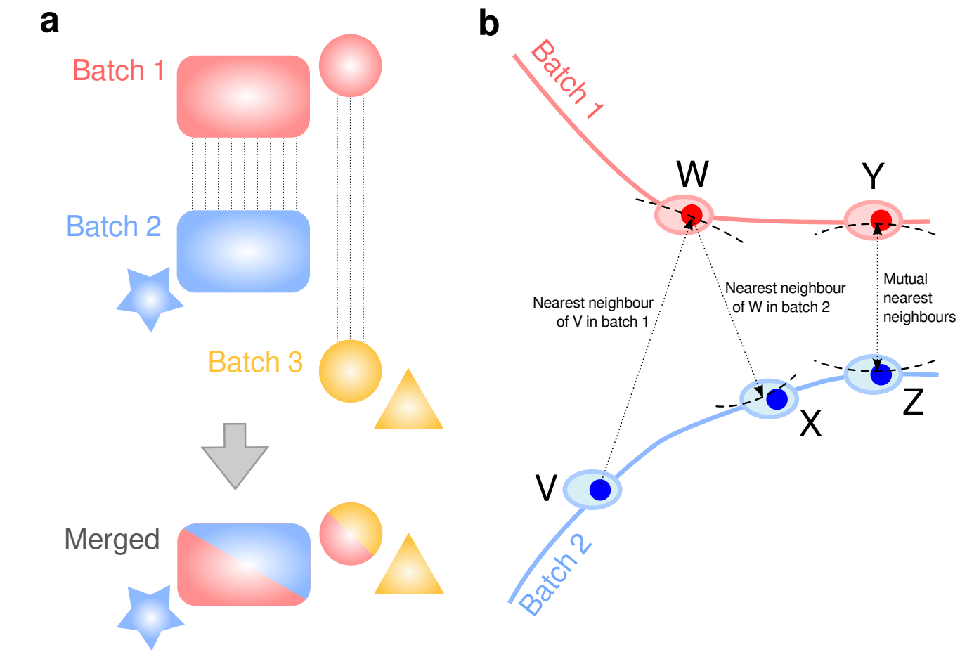
Figure 14.1: mnnCorrect batch/dataset effect correction. From Haghverdi et al. 2017
is.common <- rowData(muraro)$feature_symbol %in% rowData(segerstolpe)$feature_symbol
muraro <- muraro[is.common,]
segerstolpe <- segerstolpe[match(rowData(muraro)$feature_symbol, rowData(segerstolpe)$feature_symbol),]
rownames(segerstolpe) <- rowData(segerstolpe)$feature_symbol
rownames(muraro) <- rowData(muraro)$feature_symbol
identical(rownames(segerstolpe), rownames(muraro))## [1] TRUElibrary("batchelor")
identical(rownames(muraro), rownames(segerstolpe))
# mnnCorrect will take several minutes to run
corrected <- mnnCorrect(logcounts(muraro), logcounts(segerstolpe), k=20)First let’s check that we found a sufficient number of mnn pairs, mnnCorrect returns a list of dataframe with the mnn pairs for each dataset.
The first and second columns contain the cell column IDs and the third column contains a number indicating which dataset/batch the column 2 cell belongs to. In our case, we are only comparing two datasets so all the mnn pairs have been assigned to the second table and the third column contains only ones
head(corrected$pairs[[2]])
total_pairs <- nrow(corrected$pairs[[2]])
n_unique_seger <- length(unique((corrected$pairs[[2]][,1])))
n_unique_muraro <- length(unique((corrected$pairs[[2]][,2])))mnnCorrect found “r total_pairs” sets of mutual nearest-neighbours between
n_unique_seger segerstolpe cells and n_unique_muraro muraro cells. This
should be a sufficient number of pairs but the low number of unique cells in
each dataset suggests we might not have captured the full biological signal in
each dataset.
Exercise Which cell-types had mnns across these datasets? Should we increase/decrease k?
Answer
Now we could create a combined dataset to jointly analyse these data. However, the corrected data is no longer counts and usually will contain negative expression values thus some analysis tools may no longer be appropriate. For simplicity let’s just plot a joint TSNE.
library("Rtsne")
joint_expression_matrix <- cbind(corrected$corrected[[1]], corrected$corrected[[2]])
# Tsne will take some time to run on the full dataset
joint_tsne <- Rtsne(t(joint_expression_matrix[rownames(joint_expression_matrix) %in% var.genes,]), initial_dims=10, theta=0.75,
check_duplicates=FALSE, max_iter=200, stop_lying_iter=50, mom_switch_iter=50)
dataset_labels <- factor(rep(c("m", "s"), times=c(ncol(muraro), ncol(segerstolpe))))
cell_type_labels <- factor(c(colData(muraro)$cell_type1, colData(segerstolpe)$cell_type1))
plot(joint_tsne$Y[,1], joint_tsne$Y[,2], pch=c(16,1)[dataset_labels], col=rainbow(length(levels(cell_type_labels)))[cell_type_labels])14.6 “Anchor” integration (Seurat)
The Seurat package originally proposed another correction method for combining multiple datasets, called CCA. However, unlike mnnCorrect it doesn’t correct the expression matrix itself directly. Instead Seurat finds a lower dimensional subspace for each dataset then corrects these subspaces. Also different from mnnCorrect, Seurat could only combine a single pair of datasets at a time with CCA.
Recently, the Seurat team proposed a new method to integrate single-cell datasets using “anchors” (???).
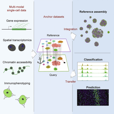
Figure 14.2: Seurat integration with anchors.
Note: because Seurat uses up a lot of library space you may need to restart your R-session to load it, and the plots/output won’t be automatically generated on this page. Also the analysis presented below is relatively time and memory consuming. As such, we have not run these commands when compiling this website and therefore no output is shown here. Approach with caution if you are trying to run this analysis on a laptop!
Reload the data:
muraro <- readRDS("data/pancreas/muraro.rds")
segerstolpe <- readRDS("data/pancreas/segerstolpe.rds")
segerstolpe <- segerstolpe[,colData(segerstolpe)$cell_type1 != "unclassified"]
segerstolpe <- segerstolpe[,colData(segerstolpe)$cell_type1 != "not applicable",]
muraro <- muraro[,colData(muraro)$cell_type1 != "unclear"]
is.common <- rowData(muraro)$feature_symbol %in% rowData(segerstolpe)$feature_symbol
muraro <- muraro[is.common,]
segerstolpe <- segerstolpe[match(rowData(muraro)$feature_symbol, rowData(segerstolpe)$feature_symbol),]
rownames(segerstolpe) <- rowData(segerstolpe)$feature_symbol
rownames(muraro) <- rowData(muraro)$feature_symbol
identical(rownames(segerstolpe), rownames(muraro))First we will reformat our data into Seurat objects:
library("Seurat")
library(scater)
library(SingleCellExperiment)
set.seed(4719364)
muraro_seurat <- CreateSeuratObject(normcounts(muraro)) # raw counts aren't available for muraro
muraro_seurat@meta.data[, "dataset"] <- 1
muraro_seurat@meta.data[, "celltype"] <- paste("m",colData(muraro)$cell_type1, sep="-")
seger_seurat <- CreateSeuratObject(counts(segerstolpe))
seger_seurat@meta.data[, "dataset"] <- 2
seger_seurat@meta.data[, "celltype"] <- paste("s",colData(segerstolpe)$cell_type1, sep="-")Next we must normalize, scale and identify highly variable genes for each dataset:
muraro_seurat <- NormalizeData(object=muraro_seurat)
muraro_seurat <- ScaleData(object=muraro_seurat)
muraro_seurat <- FindVariableFeatures(object=muraro_seurat)

seger_seurat <- NormalizeData(object=seger_seurat)
seger_seurat <- ScaleData(object=seger_seurat)
seger_seurat <- FindVariableFeatures(object=seger_seurat)
Even though Seurat corrects for the relationship between dispersion and mean expression, it doesn’t use the corrected value when ranking features. Compare the results of the command below with the results in the plots above:
Next, we use the SelectIntegrationFeatures function to select with genes to
use to integrate the two datasets here.
seurat_list <- list(muraro = muraro_seurat, seger = seger_seurat)
features <- SelectIntegrationFeatures(object.list = seurat_list)
seurat_list <- lapply(X = seurat_list, FUN = function(x) {
  x <- ScaleData(x, features = features, verbose = FALSE)
  x <- RunPCA(x, features = features, verbose = FALSE)
})
Now we will run FindIntegrationAnchors and then IntegrateData to integrate
the datasets:
pancreas.anchors <- FindIntegrationAnchors(object.list = seurat_list, dims = 1:30)

pancreas.integrated <- IntegrateData(anchorset = pancreas.anchors, dims = 1:30)
To view the output of the integration we could run the following plotting commands.
library(ggplot2)
library(cowplot)
                                        # switch to integrated assay. The variable features of this assay are automatically
                                        # set during IntegrateData
DefaultAssay(pancreas.integrated) <- "integrated"

                                        # Run the standard workflow for visualization and clustering
pancreas.integrated <- ScaleData(pancreas.integrated, verbose = FALSE)
pancreas.integrated <- RunPCA(pancreas.integrated, npcs = 30, verbose = FALSE)
pancreas.integrated <- RunUMAP(pancreas.integrated, reduction = "pca", dims = 1:30)
p1 <- DimPlot(pancreas.integrated, reduction = "umap", group.by = "dataset")
p2 <- DimPlot(pancreas.integrated, reduction = "umap", group.by = "celltype", label = TRUE,
              repel = TRUE) + NoLegend()
plot_grid(p1, p2)
Q: How well do you think this approach integrates these two pancreatic datasets?
Advanced Exercise Use the clustering methods we previously covered on the combined datasets. Do you identify any novel cell-types?
For more details on using Seurat for this type of analysis, please consult the relevant vignettes and documentation
14.7 Search scRNA-Seq data
14.7.1 About
scfind is a tool that allows one to search single cell RNA-Seq collections
(Atlas) using lists of genes, e.g. searching for cells and cell-types where a
specific set of genes are expressed. scfind is a Github
package. Cloud implementation of
scfind with a large collection of datasets is available on our
website.
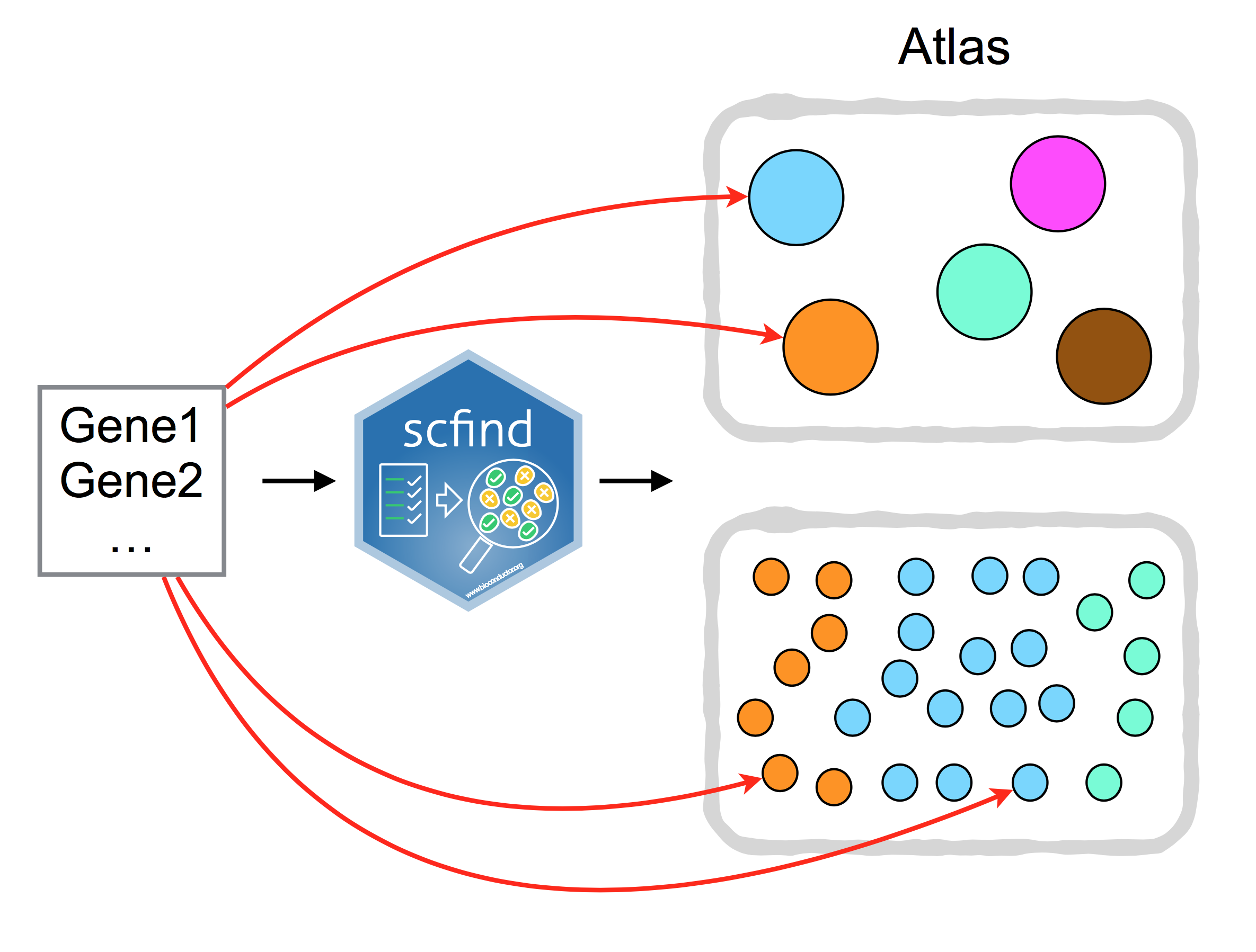
Figure 14.3: scfind can be used to search large collection of scRNA-seq data by a list of gene IDs.
14.7.2 Dataset
We will run scfind on the Tabula Muris 10X dataset. scfind also operates on
SingleCellExperiment class:
tm10x_heart <- readRDS("data/sce/Heart_10X.rds")
tm10x_heart <- tm10x_heart[, !is.na(tm10x_heart$cell_type1)]
tm10x_heart
## class: SingleCellExperiment
## dim: 23341 624
## metadata(1): log.exprs.offset
## assays(3): counts normcounts logcounts
## rownames(23341): Xkr4 Rp1 ... Tdtom_transgene zsGreen_transgene
## rowData names(1): feature_symbol
## colnames(624): 10X_P7_4_AAACCTGCACGACGAA-1
## 10X_P7_4_AAACCTGGTTCCACGG-1 ... 10X_P7_4_TTTGTCAGTCGATTGT-1
## 10X_P7_4_TTTGTCAGTGCGCTTG-1
## colData names(5): mouse cell_type1 tissue subtissue sex
## reducedDimNames(3): UMAP PCA TSNE
## spikeNames(0):## DataFrame with 624 rows and 5 columns
## mouse cell_type1 tissue
## <factor> <factor> <factor>
## 10X_P7_4_AAACCTGCACGACGAA-1 3-F-56 endothelial cell Heart
## 10X_P7_4_AAACCTGGTTCCACGG-1 3-F-56 fibroblast Heart
## 10X_P7_4_AAACCTGTCTCGATGA-1 3-F-56 endothelial cell Heart
## 10X_P7_4_AAACGGGAGCGCTCCA-1 3-F-56 cardiac muscle cell Heart
## 10X_P7_4_AAAGCAAAGTGAATTG-1 3-F-56 fibroblast Heart
## ... ... ... ...
## 10X_P7_4_TTTGGTTCAGACTCGC-1 3-F-56 cardiac muscle cell Heart
## 10X_P7_4_TTTGTCAAGTGGAGAA-1 3-F-56 cardiac muscle cell Heart
## 10X_P7_4_TTTGTCACAAGCCATT-1 3-F-56 endocardial cell Heart
## 10X_P7_4_TTTGTCAGTCGATTGT-1 3-F-56 endothelial cell Heart
## 10X_P7_4_TTTGTCAGTGCGCTTG-1 3-F-56 fibroblast Heart
## subtissue sex
## <factor> <factor>
## 10X_P7_4_AAACCTGCACGACGAA-1 NA F
## 10X_P7_4_AAACCTGGTTCCACGG-1 NA F
## 10X_P7_4_AAACCTGTCTCGATGA-1 NA F
## 10X_P7_4_AAACGGGAGCGCTCCA-1 NA F
## 10X_P7_4_AAAGCAAAGTGAATTG-1 NA F
## ... ... ...
## 10X_P7_4_TTTGGTTCAGACTCGC-1 NA F
## 10X_P7_4_TTTGTCAAGTGGAGAA-1 NA F
## 10X_P7_4_TTTGTCACAAGCCATT-1 NA F
## 10X_P7_4_TTTGTCAGTCGATTGT-1 NA F
## 10X_P7_4_TTTGTCAGTGCGCTTG-1 NA F14.7.3 Cell type search
If one has a list of genes that you would like to check against you dataset, i.e. find the cell types that most likely represent your genes (highest expression), then scfind allows one to do that by first creating a gene index and then very quickly searching the index.
The input data for indexing is the raw count matrix of the
SingleCellExperiment class. By default the cell_type1 column of the
colData slot of the SingleCellExperiment object is used to define cell
types, however it can also be defined manually using the cell.type.label
argument of the buildCellTypeIndex.
scfind adopts a two-step compression strategy which allows efficient
compression of large cell-by-gene matrix and allows fast retrieval of data by
gene query. The authors estimated that one can achieve 2 orders of magnitude
compression with this method.
We can look at the p-values from scfind to discover the best matches.
p_values <- -log10(findCellType(heart_index, c("Fstl1")))
barplot(p_values, ylab = "-log10(pval)", las = 2)
Exercise: Search for some of your favourite genes in the heart data!
Exercise: Repeat this approach to build a cell type index for the thymus data.
tm10x_thymus <- readRDS("data/sce/Thymus_10X.rds")
tm10x_thymus <- tm10x_thymus[, !is.na(tm10x_thymus$cell_type1)]
thymus_index <- buildCellTypeIndex(
  tm10x_thymus,
  cell_type_column   = "cell_type1"
)

p_values <- -log10(findCellType(thymus_index, c("Cd74")))
barplot(p_values, ylab = "-log10(pval)", las = 2)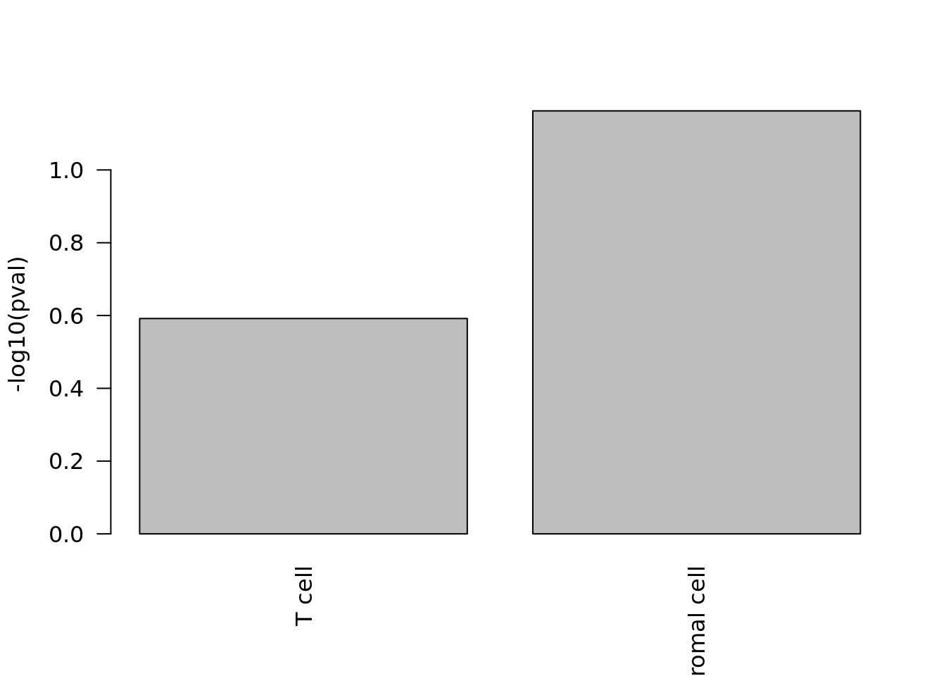
Exercise: Search for interesting genes in the thymus data!
14.7.4 Cell search
If one is more interested in finding out in which cells all the genes from your gene list are expressed in, then you can build a cell index instead of a cell type index. buildCellIndex function should be used for building the index and findCell for searching the index:
heart_gene_index <- buildCellIndex(tm10x_heart)
res <- findCell(heart_gene_index, c("Fstl1", "Ppia"))
head(res$common_exprs_cells)
## cell_id cell_type
## 1 1 endothelial cell
## 2 2 fibroblast
## 3 7 fibroblast
## 4 9 endocardial cell
## 5 10 smooth muscle cell
## 6 13 smooth muscle cell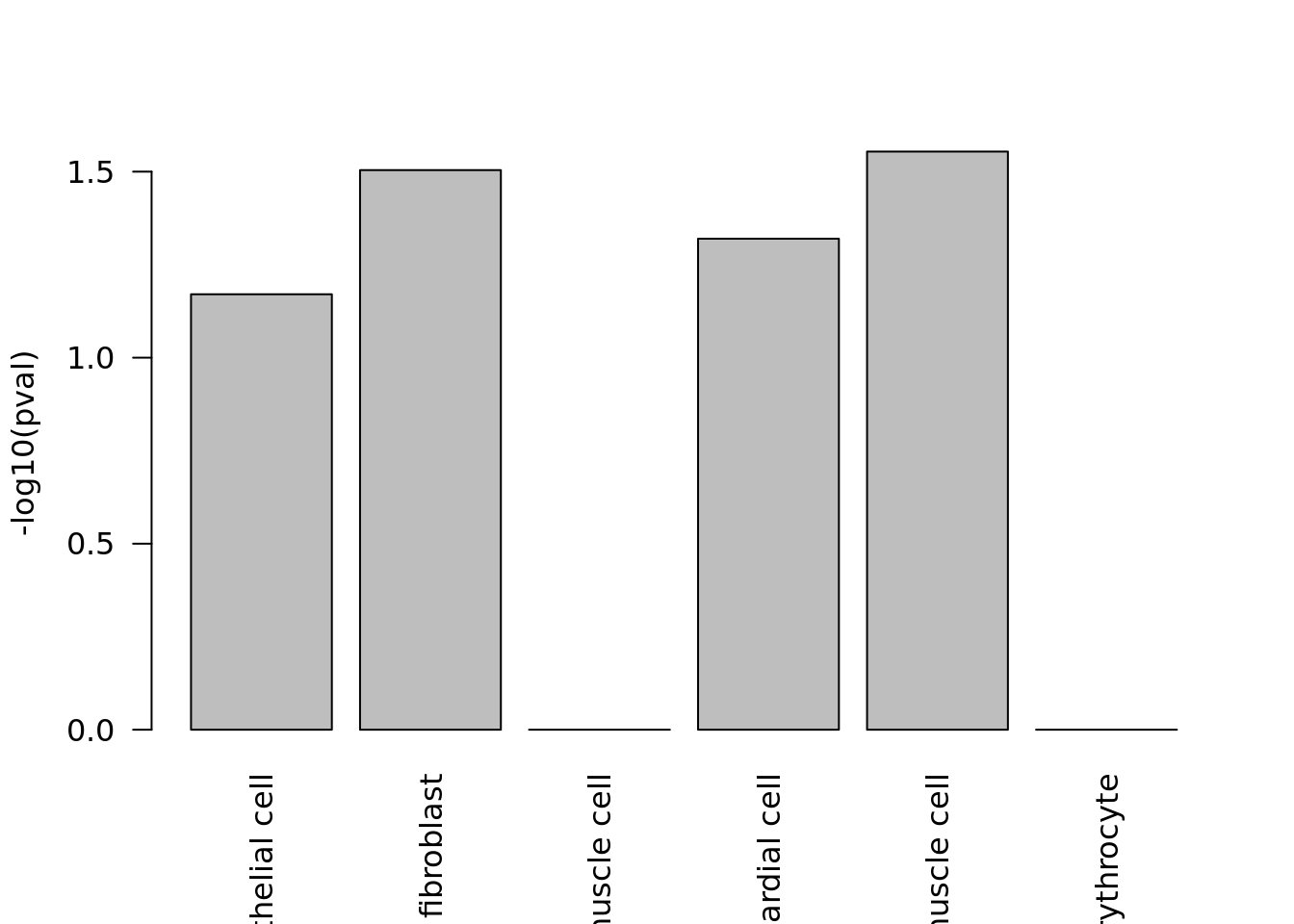
Cell search reports the p-values corresponding to cell types as well.
Exercise: Search for some of your favourite genes in the heart data!
Exercise: Repeat this approach to build a cell type index for the thymus data.
Advanced exercise: Try scfind on the Deng data and see if you can find
interesting results for well-known developmental genes in that mouse embryo
data.
14.7.5 Explore
Exercise: Play around with the scfind website, which allow for searching of several large “atlas”-type datasets. This could be a useful way to check the utility or validity of cell-type marker genes before use in your own analysis.
For example, you might explore the following cardiac contractility genes in the Mouse Atlas or Tabula Muris datasets.
14.7.5.1 In-silico gating
On the scfind website, you can perform “in-silico gating” using logical operators on marker genes to identify cell type subsets similar to the cell sorting works. To do so, you can add logical operators including “-” and "*" for “no” and “intermediate” expression, respectively in front of the gene name.
Exercise: Try out some in silico gating on one or more datasets available at the scfind website. For example, can you gate to find regulatory T cells and effector memory T cells?
14.7.6 sessionInfo()
## R version 3.6.0 (2019-04-26)
## Platform: x86_64-pc-linux-gnu (64-bit)
## Running under: Ubuntu 18.04.3 LTS
##
## Matrix products: default
## BLAS:   /usr/lib/x86_64-linux-gnu/blas/libblas.so.3.7.1
## LAPACK: /usr/lib/x86_64-linux-gnu/lapack/liblapack.so.3.7.1
##
## locale:
##  [1] LC_CTYPE=en_AU.UTF-8       LC_NUMERIC=C
##  [3] LC_TIME=en_AU.UTF-8        LC_COLLATE=en_AU.UTF-8
##  [5] LC_MONETARY=en_AU.UTF-8    LC_MESSAGES=en_AU.UTF-8
##  [7] LC_PAPER=en_AU.UTF-8       LC_NAME=C
##  [9] LC_ADDRESS=C               LC_TELEPHONE=C
## [11] LC_MEASUREMENT=en_AU.UTF-8 LC_IDENTIFICATION=C
##
## attached base packages:
## [1] parallel  stats4    stats     graphics  grDevices utils     datasets
## [8] methods   base
##
## other attached packages:
##  [1] plotly_4.9.0                scfind_1.6.0
##  [3] scmap_1.6.0                 scater_1.12.2
##  [5] ggplot2_3.2.1               SingleCellExperiment_1.6.0
##  [7] SummarizedExperiment_1.14.1 DelayedArray_0.10.0
##  [9] BiocParallel_1.18.1         matrixStats_0.55.0
## [11] Biobase_2.44.0              GenomicRanges_1.36.1
## [13] GenomeInfoDb_1.20.0         IRanges_2.18.3
## [15] S4Vectors_0.22.1            BiocGenerics_0.30.0
## [17] googleVis_0.6.4
##
## loaded via a namespace (and not attached):
##  [1] httr_1.4.1               viridis_0.5.1
##  [3] tidyr_1.0.0              BiocSingular_1.0.0
##  [5] jsonlite_1.6             viridisLite_0.3.0
##  [7] DelayedMatrixStats_1.6.1 assertthat_0.2.1
##  [9] highr_0.8                GenomeInfoDbData_1.2.1
## [11] vipor_0.4.5              yaml_2.2.0
## [13] backports_1.1.4          pillar_1.4.2
## [15] lattice_0.20-38          glue_1.3.1
## [17] digest_0.6.21            XVector_0.24.0
## [19] randomForest_4.6-14      colorspace_1.4-1
## [21] htmltools_0.3.6          Matrix_1.2-17
## [23] plyr_1.8.4               pkgconfig_2.0.3
## [25] bookdown_0.13            zlibbioc_1.30.0
## [27] purrr_0.3.2              scales_1.0.0
## [29] tibble_2.1.3             proxy_0.4-23
## [31] withr_2.1.2              lazyeval_0.2.2
## [33] magrittr_1.5             crayon_1.3.4
## [35] evaluate_0.14            class_7.3-15
## [37] beeswarm_0.2.3           tools_3.6.0
## [39] hash_2.2.6.1             data.table_1.12.2
## [41] lifecycle_0.1.0          stringr_1.4.0
## [43] munsell_0.5.0            irlba_2.3.3
## [45] compiler_3.6.0           e1071_1.7-2
## [47] rsvd_1.0.2               rlang_0.4.0
## [49] grid_3.6.0               RCurl_1.95-4.12
## [51] BiocNeighbors_1.2.0      htmlwidgets_1.3
## [53] bitops_1.0-6             labeling_0.3
## [55] rmarkdown_1.15           gtable_0.3.0
## [57] codetools_0.2-16         reshape2_1.4.3
## [59] R6_2.4.0                 gridExtra_2.3
## [61] knitr_1.25               dplyr_0.8.3
## [63] zeallot_0.1.0            bit_1.1-14
## [65] stringi_1.4.3            ggbeeswarm_0.6.0
## [67] Rcpp_1.0.2               vctrs_0.2.0
## [69] tidyselect_0.2.5         xfun_0.9
References
Altschul, Stephen F., Warren Gish, Webb Miller, Eugene W. Myers, and David J. Lipman. 1990. “Basic Local Alignment Search Tool.” Journal of Molecular Biology 215 (3). Elsevier BV: 403–10. https://doi.org/10.1016/s0022-2836(05)80360-2.
Kiselev, Vladimir Yu, and Martin Hemberg. 2017. “Scmap - a Tool for Unsupervised Projection of Single Cell RNA-seq Data.” bioRxiv, July, 150292.
Muraro, Mauro J., Gitanjali Dharmadhikari, Dominic Grün, Nathalie Groen, Tim Dielen, Erik Jansen, Leon van Gurp, et al. 2016. “A Single-Cell Transcriptome Atlas of the Human Pancreas.” Cell Systems 3 (4). Elsevier BV: 385–394.e3. https://doi.org/10.1016/j.cels.2016.09.002.
Regev, Aviv, Sarah Teichmann, Eric S Lander, Ido Amit, Christophe Benoist, Ewan Birney, Bernd Bodenmiller, et al. 2017. “The Human Cell Atlas.” bioRxiv, May, 121202.
Segerstolpe, Åsa, Athanasia Palasantza, Pernilla Eliasson, Eva-Marie Andersson, Anne-Christine Andréasson, Xiaoyan Sun, Simone Picelli, et al. 2016. “Single-Cell Transcriptome Profiling of Human Pancreatic Islets in Health and Type 2 Diabetes.” Cell Metabolism 24 (4). Elsevier BV: 593–607. https://doi.org/10.1016/j.cmet.2016.08.020.