7 Normalization, confounders and batch correction
7.1 Normalization theory
7.1.1 Introduction
In this chapter, we will explore approaches to normalization, confounder identification and batch correction for scRNA-seq data.
Even in the absence of specific confounding factors, thoughtful normalization of scRNA-seq data is required. The raw count values are not directly comparable between cells, because in general the sequencing depth (number of reads obtained; often called library size) is very different across cells—orders-of-magnitude differences in sequencing depth are commonly observed between cells in an scRNA-seq dataset. If ignored, or not handled correctly, library size differences can be the dominant source of variation between single-cell gene expression profiles, obscuring the biological signal of interest. n Related to library size, differences in library composition can also cause problems when we are trying to compare expression profiles between cells. Normalization can and should also account for differences in library composition.
In addition to normalization, it is also useful to identify confounding factors so that they can be accounted for in downstream analyses. In many cases, “accounting” for confounding variables may involve incorporating them as variables in a particular statistical model (e.g. in a differential expression model). In other cases, it may be desirable to “regress out” (either in a literal or figurative sense) confounding factors—the challenge for scRNA-seq data is finding the right model and/or data transformation such that regressing out confounding factors would work as desired. We discuss this further below.
The issue of batch effects is just as important for scRNA-seq data as it is in other areas of genomics. Briefly, scRNA-seq and other ’omics assays are sensitive to minor differences in technical features of data generation. As such, even when assaying the same experimental or biological system, measurements taken at difference times and places or by different people will differ substantially. To make valid comparisons between cells, samples or groups, we first need to design our studies to be robust to batch effects and then we need to treat batch effects appropriately in our analyses.
In the following sections, we will explore simple size-factor normalizations correcting for library size and composition and also discuss a more recent, conceptually quite different, approach to tackling the problem of library size differences between cells.
7.1.2 Library size
Library sizes vary because scRNA-seq data is often sequenced on highly multiplexed platforms the total reads which are derived from each cell may differ substantially.
Most scRNA-seq platforms and/or quantification methods currently available produce count values as the “raw”, “observed”, gene expression values. For such count data, the library size must be corrected for as part of data normalization.
One popular strategy, borrowed and extended from the analysis of bulk RNA-seq
data, is to multiply or divide each column of the expression matrix (in our
setup columns correspond to cells) by a “normalization factor” which is an
estimate of the library size relative to the other cells. Many methods to
correct for library size have been developed for bulk RNA-seq and can be equally
applied to scRNA-seq (eg. UQ, SF, CPM, RPKM, FPKM, TPM).
In addition, single-cell specific size-factor normalization methods have been
proposed to better handle the characteristics of scRNA-seq data (namely greater
sparsity/proportion of zero counts). We will demonstrate use of the size-factor
normalization method from the scran package in this chapter.
A conceptually different approach to normalization of scRNA-seq data was
proposed earlier in 2019 by (Hafemeister and Satija 2019). The idea behind the
sctransform approach is to fit a regularized negative binomial model to the
raw count data, with library size as the only explanatory variable in the model.
The residuals from this model can then be used as normalized and
variance-stabilized expression values. We show the use of this method too in
this chapter.
Some quantification methods (particularly those that quantify transcript-level
expression, e.g. Salmon,
kallisto) return
transcripts-per-million values, TPM (instead of or in addition to count values),
which effectively incorporate library size when determining gene expression
estimates and thus do not require subsequent normalization for library size.
However, TPM values may still be susceptible to library composition biases and
so normalization may still be required.
7.1.3 Scaling or size-factor normalization methods
The normalization methods discussed in this section all involve dividing the counts for each cell by a constant value to account for library size and, in some cases, library composition. These methods will typically give (adjusted/normalized) counts-per-million (CPM) or transcripts-per-million (TPM) values.
Ideally, after applying one of these scaling/size-factor normalization methods, the CPM/TPM values produced are comparable across cells, with the effects of sequencing depth removed. However, even if this is true (i.e. the normalization has worked well), the CPM/TPM values do not have stable variance. Specifically, as the size of the values increases, so does the variance. This feature of the data (heteroskedacity, or asymmetric, heavy-tailed distributions) is problematic for statistical analysis methods that assume homoskedacity, that is that there is no relationship between the mean of expression values and their variance (i.e. just about anything that uses a Gaussian error model).
As such, we should apply a variance stabilizing transformation to these data
so that we can use standard statistical methods like linear regression and PCA
with confidence. Developing a thoroughly effective variance stabilizing
transformation is a challenge, so almost universally a log transformation
(typically log2) is applied to the CPM/TPM values (the logcounts slot in a
SingleCellExperiment object is expected to contain (normalized) log2-scale
CPM/TPM values). For high-depth cells and highly-expressed genes this
transformation generally works well (as for bulk RNA-seq data), but, as we will
discuss below, it often performs sub-optimally for (sparse) scRNA-seq data.
7.1.3.1 CPM
The simplest way to normalize this data is to convert it to counts per million
(CPM) by dividing each column by its total then multiplying by 1,000,000.
Note that spike-ins should be excluded from the calculation of total expression
in order to correct for total cell RNA content, therefore we will only use
endogenous genes. Example of a CPM function in R (using the scater
package):
calc_cpm <-
function (expr_mat, spikes = NULL)
{
    norm_factor <- colSums(expr_mat[-spikes, ])
    return(t(t(expr_mat)/norm_factor)) * 10^6
}
One potential drawback of CPM is if your sample contains genes that are both very highly expressed and differentially expressed across the cells. In this case, the total molecules in the cell may depend of whether such genes are on/off in the cell and normalizing by total molecules may hide the differential expression of those genes and/or falsely create differential expression for the remaining genes.
Note RPKM, FPKM and TPM are variants on CPM which further adjust counts by the length of the respective gene/transcript. TPM is usually a direct output of a transcript expression quantification method (e.g. Salmon, kallisto, etc).
To deal with this potentiality several other measures were devised.
7.1.3.2 RLE (SF)
The size factor (SF) was proposed and popularized by DESeq (Anders and Huber 2010).
First the geometric mean of each gene across all cells is calculated. The size
factor for each cell is the median across genes of the ratio of the expression
to the gene’s geometric mean. A drawback to this method is that since it uses
the geometric mean only genes with non-zero expression values across all cells
can be used in its calculation, making it unadvisable for large low-depth
scRNASeq experiments. edgeR & scater call this method RLE for “relative
log expression” (to distinguish it from the many other size-factor normalization
methods that now exist). Example of a SF function in R (from the edgeR
package):
7.1.3.3 UQ
The upperquartile (UQ) was proposed by (Bullard et al. 2010). Here each column
is divided by the 75% quantile of the counts for each library. Often the
calculated quantile is scaled by the median across cells to keep the absolute
level of expression relatively consistent. A drawback to this method is that for
low-depth scRNASeq experiments the large number of undetected genes may result
in the 75% quantile being zero (or close to it). This limitation can be overcome
by generalizing the idea and using a higher quantile (eg. the 99% quantile is
the default in scater) or by excluding zeros prior to calculating the 75%
quantile. Example of a UQ function in R (again from the edgeR package):
7.1.3.4 TMM
Another method is called TMM is the weighted trimmed mean of M-values (to the reference) proposed by (Robinson and Oshlack 2010). The M-values in question are the gene-wise log2-fold changes between individual cells. One cell is used as the reference then the M-values for each other cell is calculated compared to this reference. These values are then trimmed by removing the top and bottom ~30%, and the average of the remaining values is calculated by weighting them to account for the effect of the log scale on variance. Each non-reference cell is multiplied by the calculated factor. Two potential issues with this method are insufficient non-zero genes left after trimming, and the assumption that most genes are not differentially expressed.
7.1.3.5 scran
scran package implements a variant on CPM size-factor normalization
specialized for single-cell data (L. Lun, Bach, and Marioni 2016). Briefly this method deals with
the problem of vary large numbers of zero values per cell by pooling cells
together calculating a normalization factor (similar to TMM) for the sum of
each pool. Since each cell is found in many different pools, cell-specific
factors can be deconvoluted from the collection of pool-specific factors using
linear algebra.
This method applies a “quick cluster” method to get rough clusters of cells to pool together to apply the strategy outlined above.
7.1.4 sctransform
The sctransform method is very different from the scaling/size-factor methods
discussed above. In their paper, (Hafemeister and Satija 2019) argue that the
log-transformation of (normalized) CPM values does not stabilise the variance of
expression values, particularly in the case of sparse(r) UMI-count data. Figure
1 of their paper (reproduced below) sets out this argument that strong
relationships exist between gene expression and total cell UMI count, even after
applying a scaled log-normalization method.
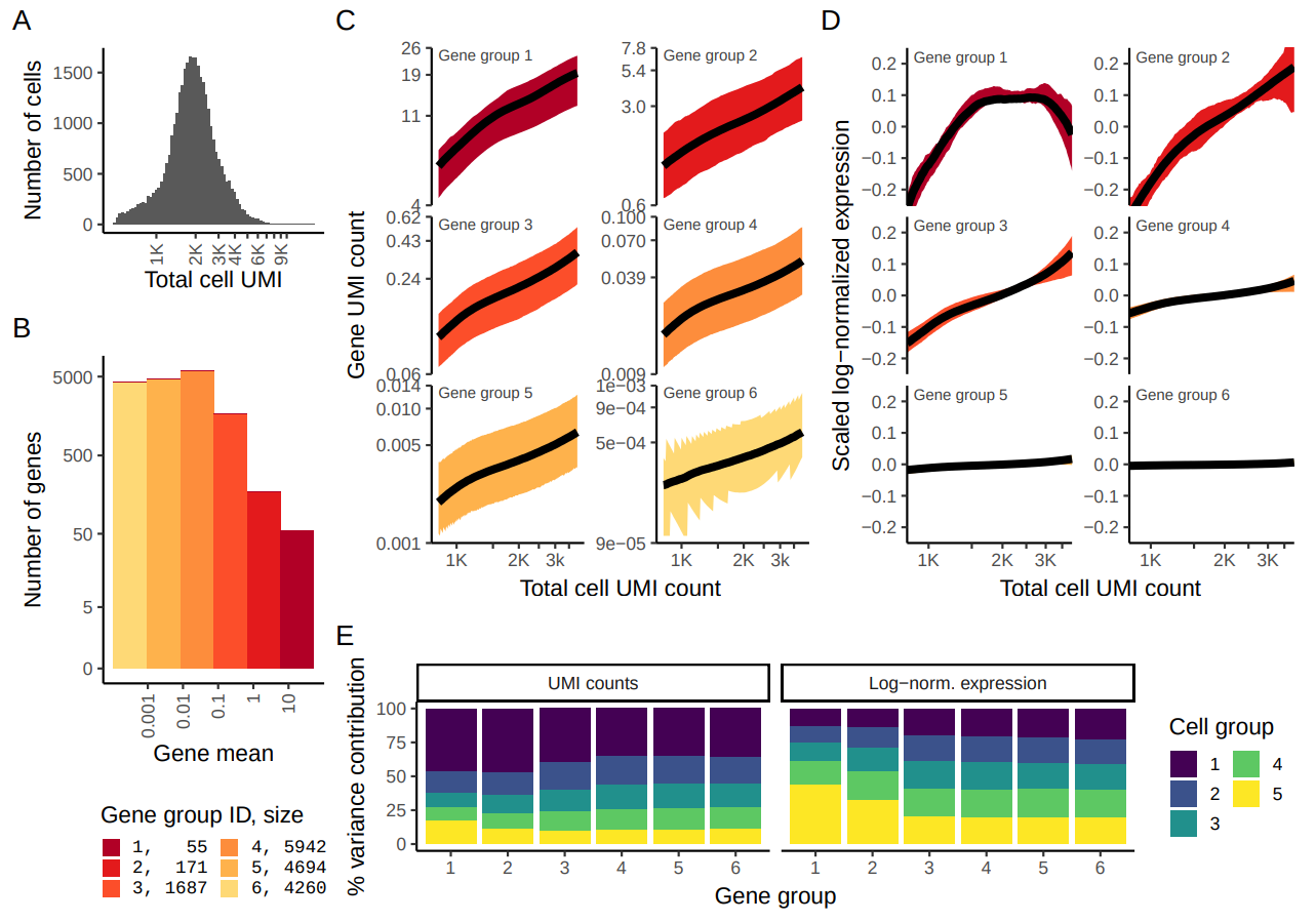
Figure 2.4: Reproduction of Figure 1 from Hafemeister and Satija (2019). 33,148 PBMC dataset from 10x genomics. A) Distribution of total UMI counts / cell (’sequencing depth’). B) We placed genesinto six groups, based on their average expression in the dataset. C) For each gene group, we examined the average relationship between observed counts and cell sequencing depth. We fit a smooth line for each gene individually and combined results based on the groupings in (B). Black line shows mean, colored region indicates interquartile range. D) Same as in (C), but showing scaled log-normalized values instead of UMI counts. Values were scaled (z-scored) so that a single y-axis range could be used. E) Relationship between gene variance and cell sequencing depth; Cells were placed into five equal-sized groups based on total UMI counts (group 1 has the greatest depth), and we calculated the total variance of each gene group within each bin. For effectively normalized data, each cell bin should contribute 20% to the variance of each gene group.
One effect of the failure of the scaled log-normalization to remove the relationship between total cell UMI count and expression is that dimension-reduction methods (especially PCA) applied to the log-normalized data can return reduced dimension spaces where, very often, the first dimension is highly correlated with total cell UMI count to total cell genes expressed. This effect is noted and discussed by (William Townes et al. 2019).
The sctransform solution is to fit a negative binomial (NB) generalized linear
model to the UMI counts for each gene, with an intercept term and a coefficient
for library size (specifically using log10(total cell UMI count) as a covariate)
as parameters in the model. The negative binomial model can account for much
more variance in the observed count data than a simpler model like the Poisson
can. To avoid overfitting the model to the data, the gene-wise intercept,
library size and overdispersion parameters are regularized by fitting a loess
(locally-linear smoothing method) to the per-gene estimates from the GLM.
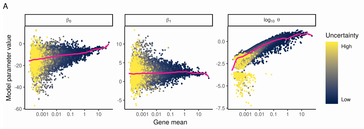
Figure 2.5: Reproduction of Figure 2A from Hafemeister and Satija (2019). They fit NB regression models for each gene individually, and bootstrapped the process to measure uncertainty in the resulting parameter estimates. A) Model parameters for 16,809 genes for the NB regression model, plotted as a function of average gene abundance. The color of each point indicates a parameter uncertainty score as determined by bootstrapping (Methods). Pink line shows the regularized parameters obtained via kernel regression.
The regularized NB GLM is presented as an attractive middle ground between the (underfit) Poisson model and the (overfit) unregularized NB model. The Pearson residuals from the regularized NB GLM are used as “normalized” expression values for downstream analyses.
![Reproduction of Figure 4 from Hafemeister and Satija (2019). A) For four genes, we show the relationship between cell sequencing depth and molecular counts. White points show the observed data. Background color represents the Pearson residual magnitude under three error models. For MALAT1 (does not vary across cell types) the Poisson error model does not account for overdispersion, and incorrectly infers significant residual variation (biological heterogeneity). For S100A9 (a CD14+ Monocyte marker) and CD74 (expressed in antigen-presenting cells) the non-regularized NB model overfits the data, and collapses biological heterogeneity. For PPBP (a Megakaryocyte marker) both non-regularized models wrongly fit a negative slope. B) Boxplot of Pearson residuals for models shown in A. X-axis range shown is limited to [-8, 25] for visual clarity.](figures/sctransform_fig5.png)
Figure 2.6: Reproduction of Figure 4 from Hafemeister and Satija (2019). A) For four genes, we show the relationship between cell sequencing depth and molecular counts. White points show the observed data. Background color represents the Pearson residual magnitude under three error models. For MALAT1 (does not vary across cell types) the Poisson error model does not account for overdispersion, and incorrectly infers significant residual variation (biological heterogeneity). For S100A9 (a CD14+ Monocyte marker) and CD74 (expressed in antigen-presenting cells) the non-regularized NB model overfits the data, and collapses biological heterogeneity. For PPBP (a Megakaryocyte marker) both non-regularized models wrongly fit a negative slope. B) Boxplot of Pearson residuals for models shown in A. X-axis range shown is limited to [-8, 25] for visual clarity.
The regularized NB GLM also provides a natural way to do feature selection ( i.e. find informative genes) using the deviance of the fitted GLM for each gene. We discuss this further in the Feature Selection section.
We find the Pearson residuals from sctransform to be highly suitable as input
to visualisation (dimension reduction) and clustering methods. For several other
analyses (e.g. differential expression analyses), where statistical models
designed for sparse count data are available, we prefer to use approaches that
work with the “raw” count data. We are not yet sure how well sctransform
performs on full-length transcript (i.e. non-UMI) count data.
7.1.5 Downsampling
A final way to correct for library size is to downsample the expression matrix so that each cell has approximately the same total number of molecules. The benefit of this method is that zero values will be introduced by the down sampling thus eliminating any biases due to differing numbers of detected genes. However, the major drawback is that the process is not deterministic so each time the downsampling is run the resulting expression matrix is slightly different. Thus, often analyses must be run on multiple downsamplings to ensure results are robust.
Downsampling to the depth of the cell with the lowest sequencing depth (that still passes QC) will typically discard much (most) of the information gathered in a (typically expensive) scRNA-seq experiment. We view this as a heavy price to pay for a normalization method that generally does not seem to outperform alternatives. Thus, we would not recommend downsampling as a normalization strategy for scRNA-seq data unless all alternatives have failed.
7.1.6 Effectiveness
To compare the efficiency of different normalization methods we will use visual
inspection of PCA plots and calculation of cell-wise relative log expression
via scater’s plotRLE() function. Namely, cells with many (few) reads have
higher (lower) than median expression for most genes resulting in a positive
(negative) RLE across the cell, whereas normalized cells have an RLE close
to zero. Example of a RLE function in R:
calc_cell_RLE <-
function (expr_mat, spikes = NULL)
{
    RLE_gene <- function(x) {
        if (median(unlist(x)) > 0) {
            log((x + 1)/(median(unlist(x)) + 1))/log(2)
        }
        else {
            rep(NA, times = length(x))
        }
    }
    if (!is.null(spikes)) {
        RLE_matrix <- t(apply(expr_mat[-spikes, ], 1, RLE_gene))
    }
    else {
        RLE_matrix <- t(apply(expr_mat, 1, RLE_gene))
    }
    cell_RLE <- apply(RLE_matrix, 2, median, na.rm = T)
    return(cell_RLE)
}
Note The RLE, TMM, and UQ size-factor methods were developed for bulk RNA-seq data and, depending on the experimental context, may not be appropriate for single-cell RNA-seq data, as their underlying assumptions may be problematically violated.
Note The calcNormFactors function from the edgeR package implements
several library size normalization methods making it easy to apply any of these
methods to our data.
Note edgeR makes extra adjustments to some of the normalization methods
which may result in somewhat different results than if the original methods are
followed exactly, e.g. edgeR’s and scater’s “RLE” method which is based on the
“size factor” used by DESeq may give
different results to the estimateSizeFactorsForMatrix method in the
DESeq/DESeq2 packages. In addition, some (earlier) versions of edgeR will
not calculate the normalization factors correctly unless lib.size is set at 1
for all cells.
Note For CPM normalisation we use scater’s calculateCPM() function.
For RLE, UQ and TMM we used to use scater’s normaliseExprs()
function, but it was deprecated and has been removed from the package). For
scran we use the scran package to calculate size factors (it also operates
on SingleCellExperiment class) and scater’s normalize() to normalise the
data. All these normalization functions save the results to the logcounts slot
of the SCE object.
7.2 Normalization practice (UMI)
We will continue to work with the tung data that was used in the previous
chapter.
library(scRNA.seq.funcs)
library(scater)
library(scran)
options(stringsAsFactors = FALSE)
set.seed(1234567)
umi <- readRDS("data/tung/umi.rds")
umi.qc <- umi[rowData(umi)$use, colData(umi)$use]
endog_genes <- !rowData(umi.qc)$is_feature_control
7.2.1 Raw
tmp <- runPCA(
  umi.qc[endog_genes, ],
  exprs_values = "logcounts_raw"
)
plotPCA(
    tmp,
    colour_by = "batch",
    size_by = "total_features_by_counts",
    shape_by = "individual"
) + ggtitle("PCA plot: raw log-counts") 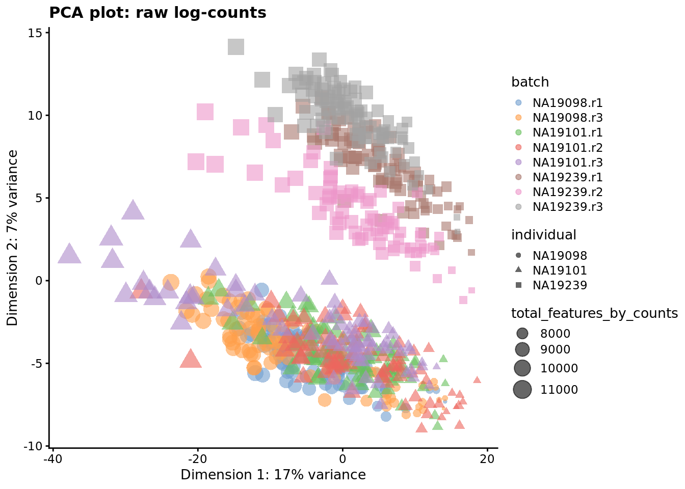
Figure 7.1: PCA plot of the tung data
7.2.2 CPM
logcounts(umi.qc) <- log2(calculateCPM(umi.qc, use_size_factors = FALSE) + 1)
plotPCA(
    umi.qc[endog_genes, ],
    colour_by = "batch",
    size_by = "total_features_by_counts",
    shape_by = "individual"
) + ggtitle("PCA plot: log2(CPM) values") 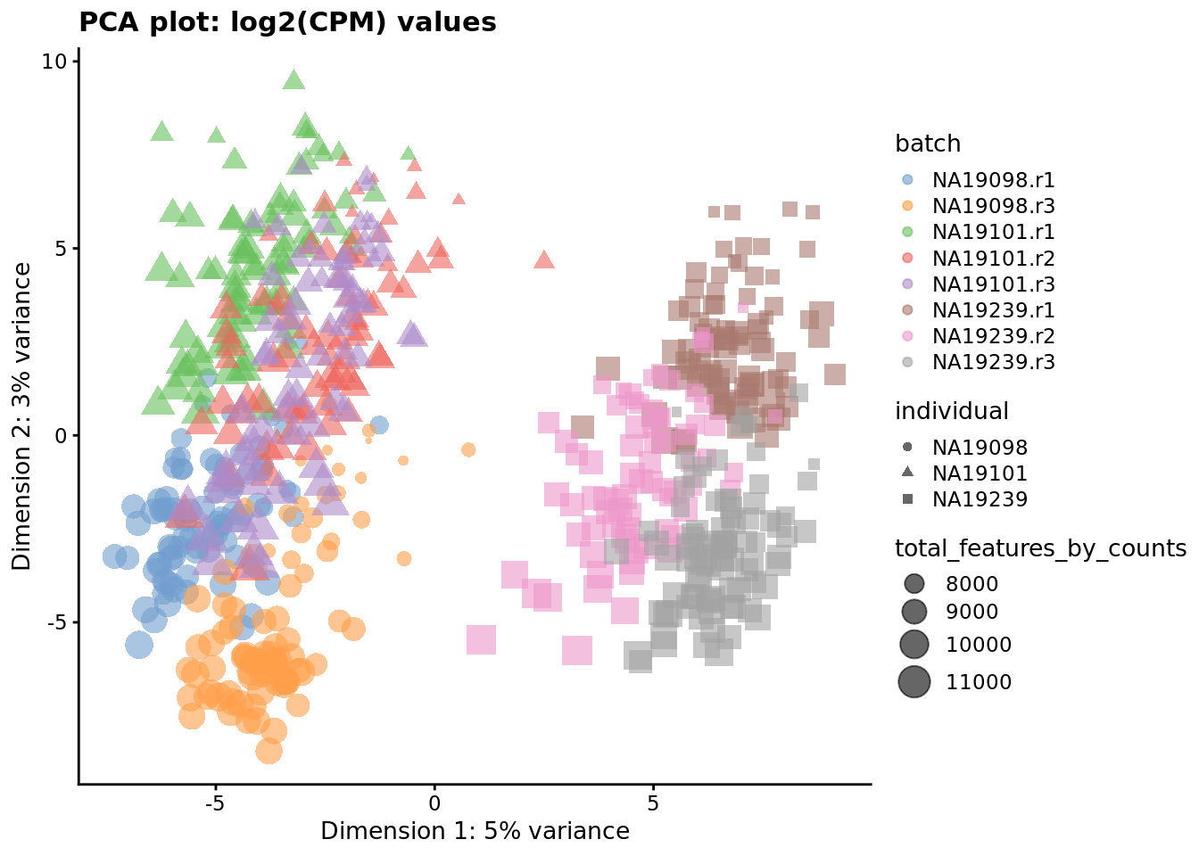
Figure 7.2: PCA plot of the tung data after CPM normalisation
plotRLE(
    umi.qc[endog_genes, ],
    exprs_values = "logcounts_raw",
    colour_by = "batch"
) + ggtitle("RLE plot: raw log-counts")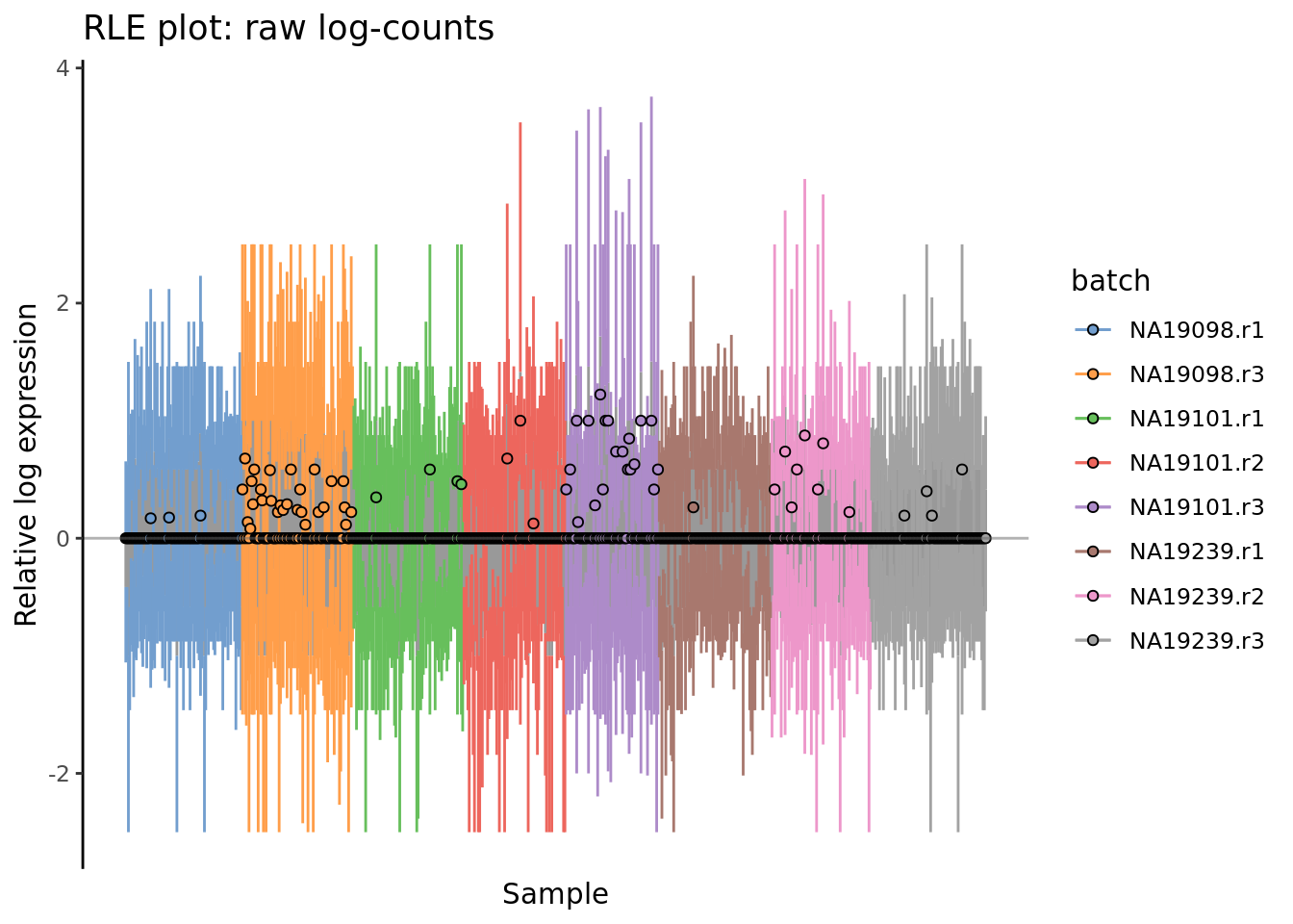
Figure 7.3: Cell-wise RLE of the tung data. The relative log expression profile of each cell is represented by a boxplot, which appears as a line here. The grey bar in the middle for each cell represent the interquartile range of the RLE values; the coloured lines represent the whiskers ofof a boxplot and extend above and below the grey bar by 1.5 times the interquartile range. The median RLE value is shown with a circle.
plotRLE(
    umi.qc[endog_genes, ],
    exprs_values = "logcounts",
    colour_by = "batch"
) + ggtitle("RLE plot: log2(CPM)")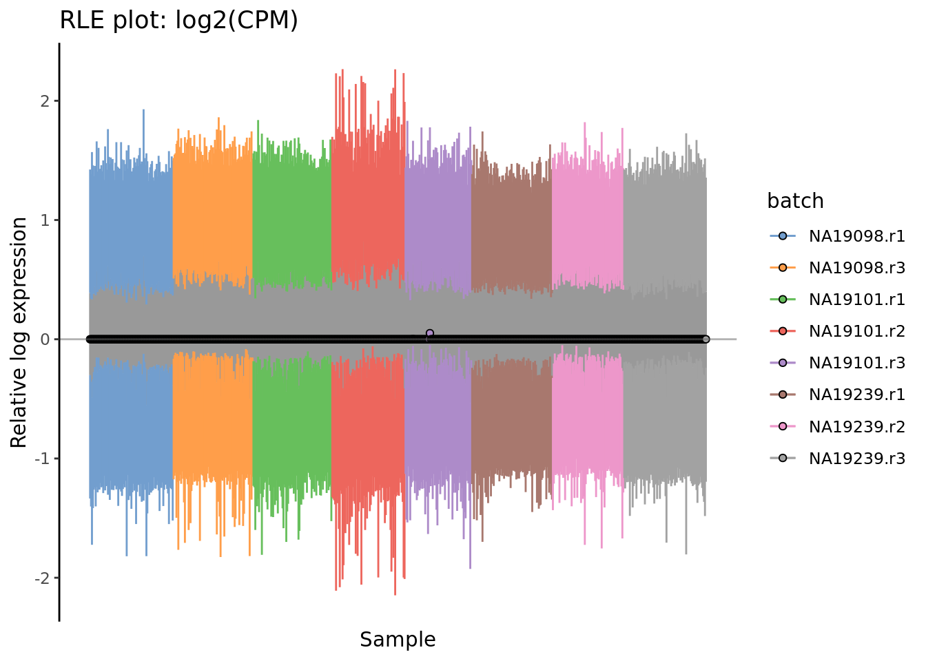
Figure 7.4: Cell-wise RLE of the tung data. The relative log expression profile of each cell is represented by a boxplot, which appears as a line here. The grey bar in the middle for each cell represent the interquartile range of the RLE values; the coloured lines represent the whiskers ofof a boxplot and extend above and below the grey bar by 1.5 times the interquartile range. The median RLE value is shown with a circle.
Q: How well would you say the two approaches above normalize the data?
7.2.3 scran
scran’s method for size-factor estimation will almost always be preferable for
scRNA-seq data to methods that were developed for bulk RNA-seq data (TMM, RLE,
UQ). Thus, we will just demonstrate the use of scran size-factor normalization
here as representative of size-factor normalization more generally.
The code below computes the size factors and then the normalize() function in
scater applies those size factors along with the library sizes to the count
matrix to produce normalized log2-counts-per-million values that are then stored
in the logcounts slot of the SingleCellExperiment object.
qclust <- quickCluster(umi.qc, min.size = 30, use.ranks = FALSE)
umi.qc <- computeSumFactors(umi.qc, sizes = 15, clusters = qclust)
umi.qc <- normalize(umi.qc)
plotPCA(
    umi.qc[endog_genes, ],
    colour_by = "batch",
    size_by = "total_features_by_counts",
    shape_by = "individual"
) + ggtitle("PCA plot: scran size-factor normalization") 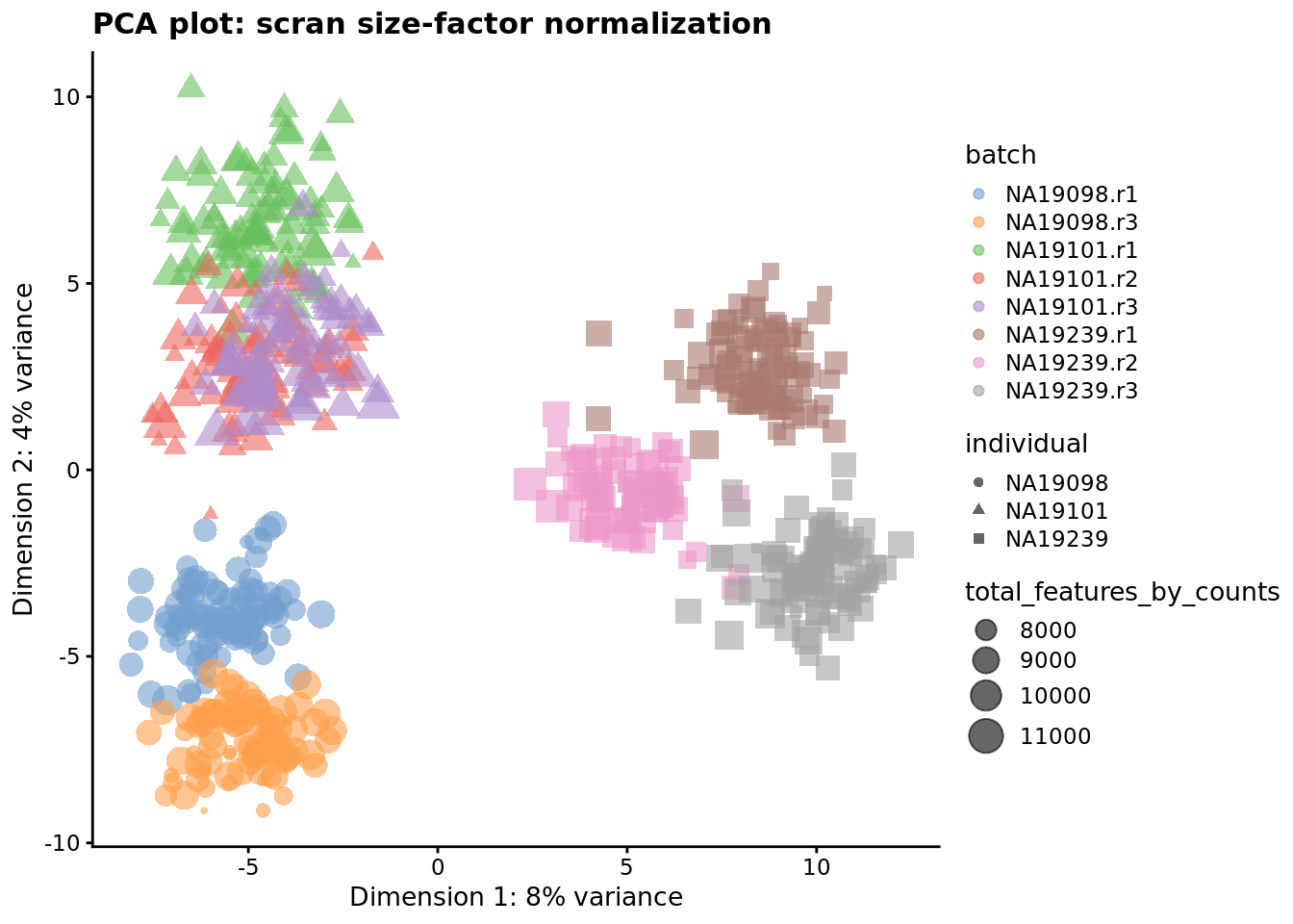
Figure 7.5: PCA plot of the tung data after LSF normalisation
plotRLE(
    umi.qc[endog_genes, ],
    exprs_values = "logcounts",
    colour_by = "batch"
) + ggtitle("RLE plot: scran size-factor normalization")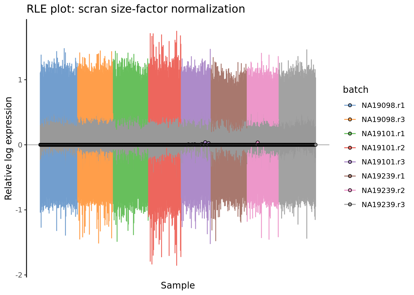
Figure 7.6: Cell-wise RLE of the tung data
scran sometimes calculates negative or zero size factors. These will
completely distort the normalized expression matrix. We can check the size
factors scran has computed like so:
##    Min. 1st Qu.  Median    Mean 3rd Qu.    Max.
##  0.4836  0.7747  0.9532  1.0000  1.1483  3.2873
For this dataset all the size factors are reasonable so we are done. If you find scran has calculated negative size factors try increasing the cluster and pool sizes until they are all positive.
We sometimes filter out cells with very large size-factors (you may like to think about why), but we will not demonstrate that here.
7.2.4 sctransform
The sctransform approach to using Pearson residuals from an regularized
negative binomial generalized linear model was introduced above. Here we
demonstrate how to apply this method.
Note that (due to what looks like a bug in this version of sctransform) we
need to convert the UMI count matrix to a sparse format to apply sctransform.
umi_sparse <- as(counts(umi.qc), "dgCMatrix")
### Genes expressed in at least 5 cells will be kept
sctnorm_data <- sctransform::vst(umi = umi_sparse, min_cells = 1,
                                 cell_attr = as.data.frame(colData(umi.qc)),
                                 latent_var = "log10_total_counts_endogenous")
## [1] 14066 657## [1] 14066 657## [1] "y ~ log10_total_counts_endogenous"Let us look at the NB GLM model parameters estimated by sctransform.
#sce$log10_total_counts
##       Matrix of estimated model parameters per gene (theta and regression coefficients)
sctransform::plot_model_pars(sctnorm_data)![]()
We can look at the effect of sctransform’s normalization on three particular genes, ACTB, POU5F1 (aka OCT4) and CD74.
##c('ACTB', 'Rpl10', 'Cd74')
genes_plot <- c("ENSG00000075624", "ENSG00000204531", "ENSG00000019582")
sctransform::plot_model(sctnorm_data, umi_sparse, genes_plot,
plot_residual = TRUE, cell_attr = as.data.frame(colData(umi.qc)))![]()
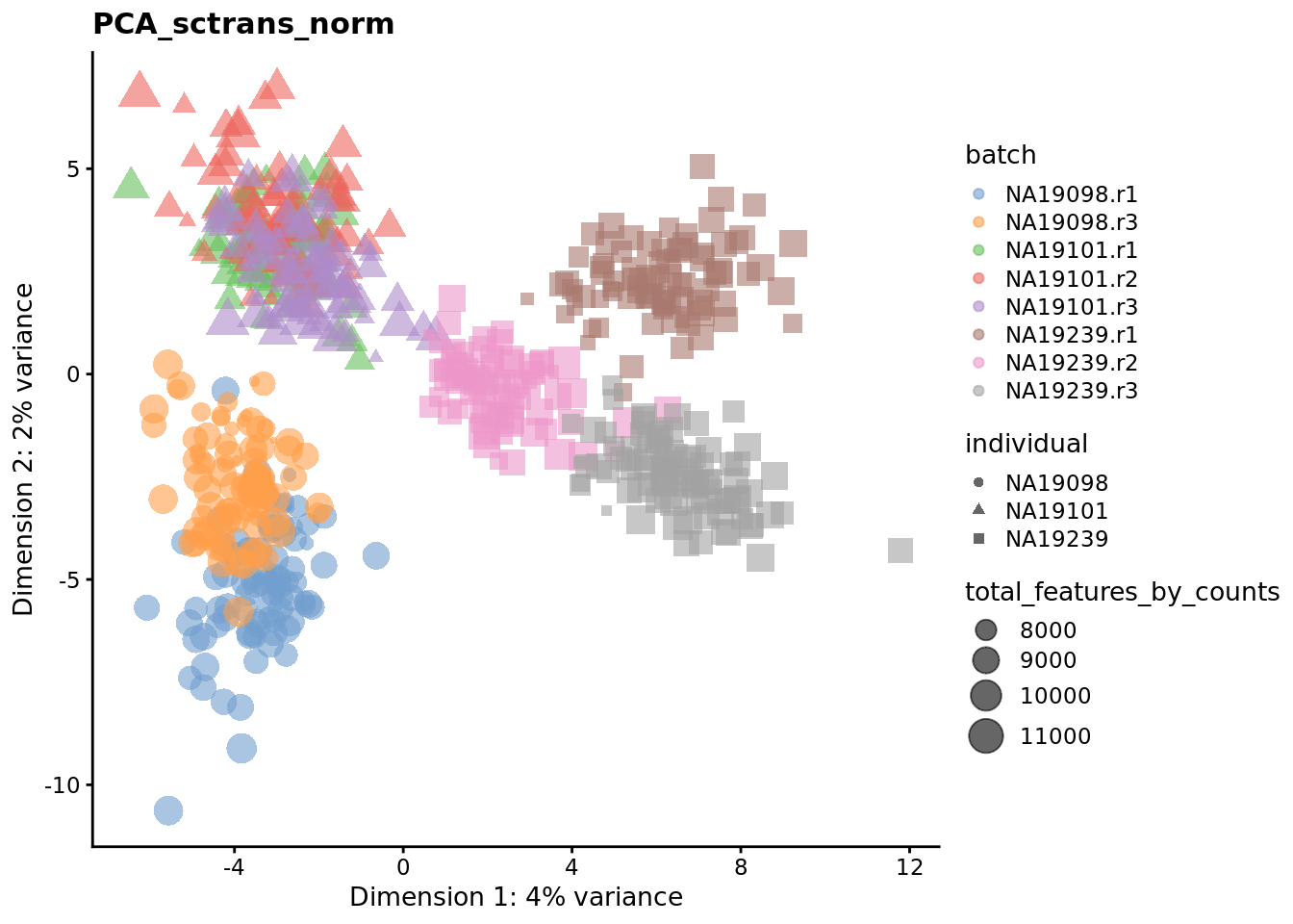
reducedDim(umi.qc, "PCA_sctrans_norm") <- reducedDim(
  runPCA(umi.qc[endog_genes, ], exprs_values = "sctrans_norm")
)
plotReducedDim(
  umi.qc,
  use_dimred = "PCA_sctrans_norm",
  colour_by = "batch",
  size_by = "total_features_by_counts",
  shape_by = "individual"
) + ggtitle("PCA plot: sctransform normalization") 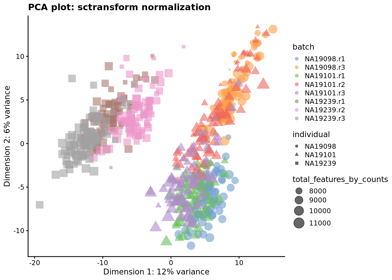
Figure 7.7: PCA plot of the tung data after sctransform normalisation (Pearson residuals).
plotRLE(
    umi.qc[endog_genes, ],
    exprs_values = "sctrans_norm",
    colour_by = "batch"
) + ggtitle("RLE plot: sctransform normalization")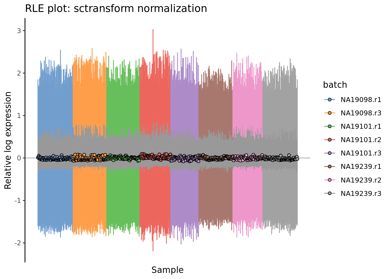
Figure 7.8: Cell-wise RLE of the tung data
7.2.5 Normalisation for gene/transcript length
Some methods combine library size and fragment/gene length normalization such as:
- RPKM - Reads Per Kilobase Million (for single-end sequencing)
- FPKM - Fragments Per Kilobase Million (same as RPKM but for paired-end sequencing, makes sure that paired ends mapped to the same fragment are not counted twice)
- TPM - Transcripts Per Kilobase Million (same as RPKM, but the order of normalizations is reversed - length first and sequencing depth second)
These methods are not applicable to our dataset since the end of the transcript which contains the UMI was preferentially sequenced. Furthermore in general these should only be calculated using appropriate quantification software from aligned BAM files not from read counts since often only a portion of the entire gene/transcript is sequenced, not the entire length. If in doubt check for a relationship between gene/transcript length and expression level.
However, here we show how these normalisations can be calculated using scater.
First, we need to find the effective transcript length in Kilobases. However,
our dataset containes only gene IDs, therefore we will be using the gene lengths
instead of transcripts. scater uses the
biomaRt
package, which allows one to annotate genes by other attributes:
umi.qc <- getBMFeatureAnnos(
    umi.qc,
    filters = "ensembl_gene_id",
    attributes = c(
        "ensembl_gene_id",
        "hgnc_symbol",
        "chromosome_name",
        "start_position",
        "end_position"
    ),
    biomart = "ENSEMBL_MART_ENSEMBL",
    dataset = "hsapiens_gene_ensembl",
    host = "www.ensembl.org"
)

# If you have mouse data, change the arguments based on this example:
# getBMFeatureAnnos(
#     object,
#     filters = "ensembl_transcript_id",
#     attributes = c(
#         "ensembl_transcript_id",
#         "ensembl_gene_id",
#         "mgi_symbol",
#         "chromosome_name",
#         "transcript_biotype",
#         "transcript_start",
#         "transcript_end",
#         "transcript_count"
#     ),
#     biomart = "ENSEMBL_MART_ENSEMBL",
#     dataset = "mmusculus_gene_ensembl",
#     host = "www.ensembl.org"
# )
Some of the genes were not annotated, therefore we filter them out:
Now we compute the total gene length in Kilobases by using the end_position
and start_position fields:
There is no relationship between gene length and mean expression so __FPKM__s & __TPM__s are inappropriate for this dataset. This is what we would expect for UMI protocols that tag one end of the transcript. But we will demonstrate them anyway.
Note Here calculate the total gene length instead of the total exon length.
Many genes will contain lots of introns so their eff_length will be very
different from what we have calculated. Please consider our calculation as
approximation. If you want to use the total exon lengths, please refer to this
page.
Now we are ready to perform the normalisations:
Plot the results as a PCA plot:
tmp <- runPCA(
  umi.qc.ann,
  exprs_values = "tpm",
)
plotPCA(
    tmp,
    colour_by = "batch",
    size_by = "total_features_by_counts",
    shape_by = "individual"
)tmp <- runPCA(
umi.qc.ann,
exprs_values = "tpm",
)
plotPCA(
tmp,
colour_by = "batch",
size_by = "total_features_by_counts",
shape_by = "individual"
)Note The PCA looks for differences between cells. Gene length is the same
across cells for each gene thus FPKM is almost identical to the CPM plot
(it is just rotated) since it performs CPM first then normalizes gene
length. Whereas, TPM is different because it weights genes by their length
before performing __CPM_**.
7.2.6 Reflection
Q: What is your assessment of the performance of these different normalization methods on the data presented here?
Q: Which normalization method would you prefer for this dataset? Why?
7.2.7 Exercise
Perform the same analysis with read counts of the tung data. Use
tung/reads.rds file to load the reads SCE object. Once you have finished
please compare your results to ours (next chapter).
7.2.8 sessionInfo()
## R version 3.6.0 (2019-04-26)
## Platform: x86_64-pc-linux-gnu (64-bit)
## Running under: Ubuntu 18.04.3 LTS
##
## Matrix products: default
## BLAS:   /usr/lib/x86_64-linux-gnu/blas/libblas.so.3.7.1
## LAPACK: /usr/lib/x86_64-linux-gnu/lapack/liblapack.so.3.7.1
##
## locale:
##  [1] LC_CTYPE=en_AU.UTF-8       LC_NUMERIC=C
##  [3] LC_TIME=en_AU.UTF-8        LC_COLLATE=en_AU.UTF-8
##  [5] LC_MONETARY=en_AU.UTF-8    LC_MESSAGES=en_AU.UTF-8
##  [7] LC_PAPER=en_AU.UTF-8       LC_NAME=C
##  [9] LC_ADDRESS=C               LC_TELEPHONE=C
## [11] LC_MEASUREMENT=en_AU.UTF-8 LC_IDENTIFICATION=C
##
## attached base packages:
## [1] parallel  stats4    stats     graphics  grDevices utils     datasets
## [8] methods   base
##
## other attached packages:
##  [1] scran_1.12.1                scater_1.12.2
##  [3] ggplot2_3.2.1               SingleCellExperiment_1.6.0
##  [5] SummarizedExperiment_1.14.1 DelayedArray_0.10.0
##  [7] BiocParallel_1.18.1         matrixStats_0.55.0
##  [9] Biobase_2.44.0              GenomicRanges_1.36.1
## [11] GenomeInfoDb_1.20.0         IRanges_2.18.3
## [13] S4Vectors_0.22.1            BiocGenerics_0.30.0
## [15] scRNA.seq.funcs_0.1.0
##
## loaded via a namespace (and not attached):
##  [1] viridis_0.5.1            dynamicTreeCut_1.63-1
##  [3] edgeR_3.26.8             BiocSingular_1.0.0
##  [5] viridisLite_0.3.0        DelayedMatrixStats_1.6.1
##  [7] elliptic_1.4-0           moments_0.14
##  [9] assertthat_0.2.1         statmod_1.4.32
## [11] highr_0.8                dqrng_0.2.1
## [13] GenomeInfoDbData_1.2.1   vipor_0.4.5
## [15] yaml_2.2.0               globals_0.12.4
## [17] pillar_1.4.2             lattice_0.20-38
## [19] glue_1.3.1               limma_3.40.6
## [21] digest_0.6.21            XVector_0.24.0
## [23] colorspace_1.4-1         plyr_1.8.4
## [25] cowplot_1.0.0            htmltools_0.3.6
## [27] Matrix_1.2-17            pkgconfig_2.0.3
## [29] listenv_0.7.0            bookdown_0.13
## [31] zlibbioc_1.30.0          purrr_0.3.2
## [33] scales_1.0.0             Rtsne_0.15
## [35] tibble_2.1.3             withr_2.1.2
## [37] lazyeval_0.2.2           magrittr_1.5
## [39] crayon_1.3.4             evaluate_0.14
## [41] future_1.14.0            MASS_7.3-51.1
## [43] beeswarm_0.2.3           tools_3.6.0
## [45] stringr_1.4.0            locfit_1.5-9.1
## [47] munsell_0.5.0            irlba_2.3.3
## [49] orthopolynom_1.0-5       compiler_3.6.0
## [51] rsvd_1.0.2               contfrac_1.1-12
## [53] rlang_0.4.0              grid_3.6.0
## [55] RCurl_1.95-4.12          BiocNeighbors_1.2.0
## [57] igraph_1.2.4.1           labeling_0.3
## [59] bitops_1.0-6             rmarkdown_1.15
## [61] codetools_0.2-16         hypergeo_1.2-13
## [63] gtable_0.3.0             deSolve_1.24
## [65] reshape2_1.4.3           R6_2.4.0
## [67] gridExtra_2.3            knitr_1.25
## [69] dplyr_0.8.3              future.apply_1.3.0
## [71] stringi_1.4.3            ggbeeswarm_0.6.0
## [73] Rcpp_1.0.2               sctransform_0.2.0
## [75] tidyselect_0.2.5         xfun_0.9
7.3 Normalization practice (Reads)
Figure 7.9: PCA plot of the tung data
Figure 7.10: PCA plot of the tung data after CPM normalisation
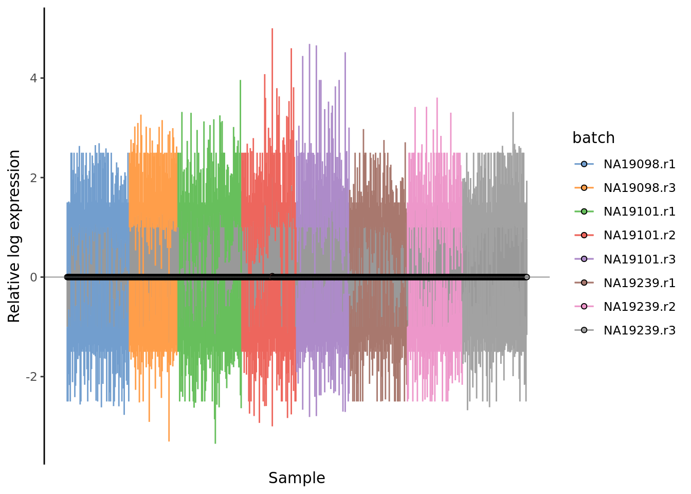
Figure 7.11: Cell-wise RLE of the tung data
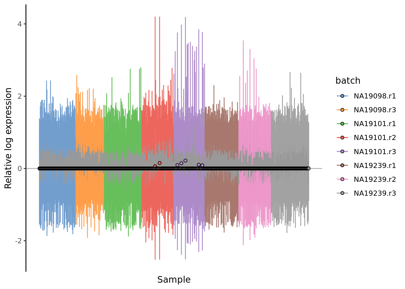
Figure 7.12: Cell-wise RLE of the tung data
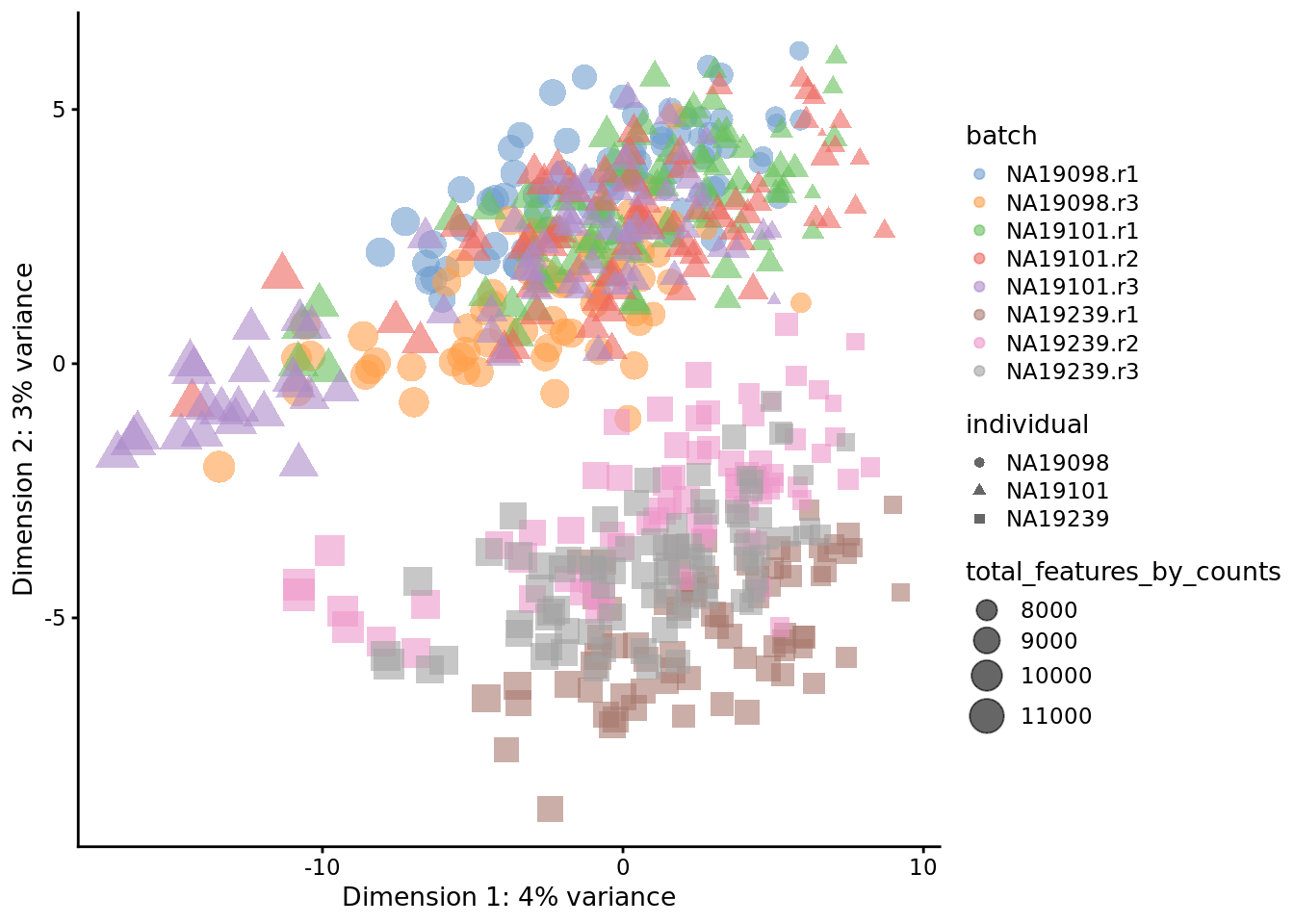
Figure 7.13: PCA plot of the tung data after LSF normalisation

Figure 7.14: Cell-wise RLE of the tung data
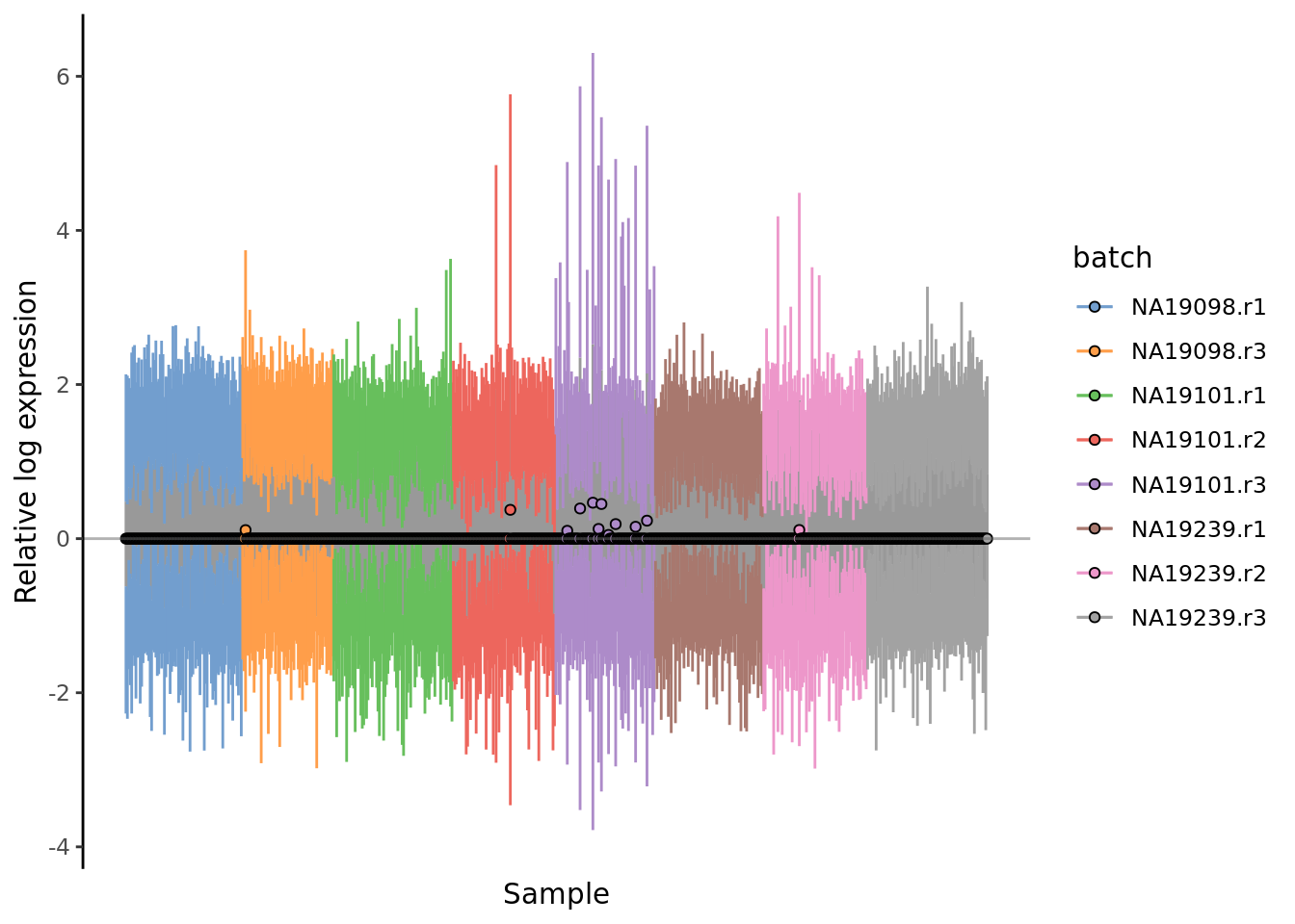
Figure 7.15: Cell-wise RLE of the tung data
Let us look at the NB GLM model parameters estimated by sctransform.
![]()
We can look at the effect of sctransform’s normalization on three particular genes, ACTB, POU5F1 (aka OCT4) and CD74.
![]()
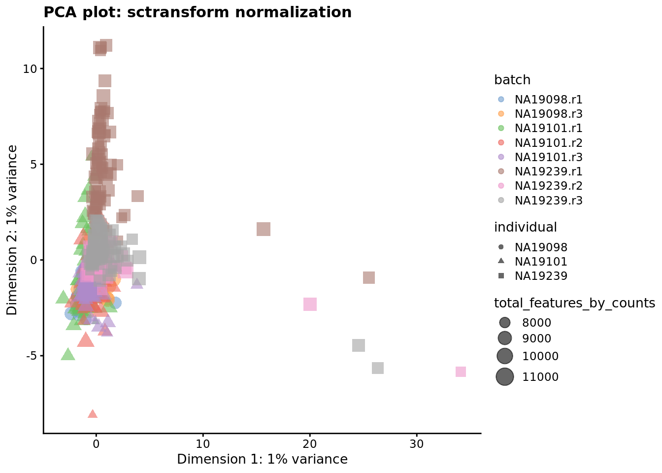
Figure 7.16: PCA plot of the tung reads data after sctransform normalisation (Pearson residuals).
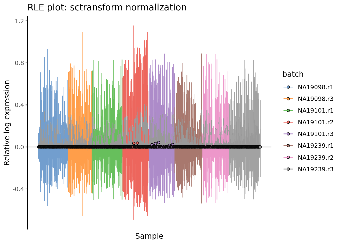
Figure 7.17: Cell-wise RLE of the tung reads data
## R version 3.6.0 (2019-04-26)
## Platform: x86_64-pc-linux-gnu (64-bit)
## Running under: Ubuntu 18.04.3 LTS
##
## Matrix products: default
## BLAS:   /usr/lib/x86_64-linux-gnu/blas/libblas.so.3.7.1
## LAPACK: /usr/lib/x86_64-linux-gnu/lapack/liblapack.so.3.7.1
##
## locale:
##  [1] LC_CTYPE=en_AU.UTF-8       LC_NUMERIC=C
##  [3] LC_TIME=en_AU.UTF-8        LC_COLLATE=en_AU.UTF-8
##  [5] LC_MONETARY=en_AU.UTF-8    LC_MESSAGES=en_AU.UTF-8
##  [7] LC_PAPER=en_AU.UTF-8       LC_NAME=C
##  [9] LC_ADDRESS=C               LC_TELEPHONE=C
## [11] LC_MEASUREMENT=en_AU.UTF-8 LC_IDENTIFICATION=C
##
## attached base packages:
## [1] parallel  stats4    stats     graphics  grDevices utils     datasets
## [8] methods   base
##
## other attached packages:
##  [1] scran_1.12.1                scater_1.12.2
##  [3] ggplot2_3.2.1               SingleCellExperiment_1.6.0
##  [5] SummarizedExperiment_1.14.1 DelayedArray_0.10.0
##  [7] BiocParallel_1.18.1         matrixStats_0.55.0
##  [9] Biobase_2.44.0              GenomicRanges_1.36.1
## [11] GenomeInfoDb_1.20.0         IRanges_2.18.3
## [13] S4Vectors_0.22.1            BiocGenerics_0.30.0
## [15] scRNA.seq.funcs_0.1.0
##
## loaded via a namespace (and not attached):
##  [1] viridis_0.5.1            dynamicTreeCut_1.63-1
##  [3] edgeR_3.26.8             BiocSingular_1.0.0
##  [5] viridisLite_0.3.0        DelayedMatrixStats_1.6.1
##  [7] elliptic_1.4-0           moments_0.14
##  [9] assertthat_0.2.1         statmod_1.4.32
## [11] highr_0.8                dqrng_0.2.1
## [13] GenomeInfoDbData_1.2.1   vipor_0.4.5
## [15] yaml_2.2.0               globals_0.12.4
## [17] pillar_1.4.2             lattice_0.20-38
## [19] glue_1.3.1               limma_3.40.6
## [21] digest_0.6.21            XVector_0.24.0
## [23] colorspace_1.4-1         plyr_1.8.4
## [25] cowplot_1.0.0            htmltools_0.3.6
## [27] Matrix_1.2-17            pkgconfig_2.0.3
## [29] listenv_0.7.0            bookdown_0.13
## [31] zlibbioc_1.30.0          purrr_0.3.2
## [33] scales_1.0.0             Rtsne_0.15
## [35] tibble_2.1.3             withr_2.1.2
## [37] lazyeval_0.2.2           magrittr_1.5
## [39] crayon_1.3.4             evaluate_0.14
## [41] future_1.14.0            MASS_7.3-51.1
## [43] beeswarm_0.2.3           tools_3.6.0
## [45] stringr_1.4.0            munsell_0.5.0
## [47] locfit_1.5-9.1           irlba_2.3.3
## [49] orthopolynom_1.0-5       compiler_3.6.0
## [51] rsvd_1.0.2               contfrac_1.1-12
## [53] rlang_0.4.0              grid_3.6.0
## [55] RCurl_1.95-4.12          BiocNeighbors_1.2.0
## [57] igraph_1.2.4.1           labeling_0.3
## [59] bitops_1.0-6             rmarkdown_1.15
## [61] codetools_0.2-16         hypergeo_1.2-13
## [63] gtable_0.3.0             deSolve_1.24
## [65] reshape2_1.4.3           R6_2.4.0
## [67] gridExtra_2.3            knitr_1.25
## [69] dplyr_0.8.3              future.apply_1.3.0
## [71] stringi_1.4.3            ggbeeswarm_0.6.0
## [73] Rcpp_1.0.2               sctransform_0.2.0
## [75] tidyselect_0.2.5         xfun_0.9
7.4 Identifying confounding factors
7.4.1 Introduction
There is a large number of potential confounders, artifacts and biases in
scRNA-seq data. One of the main challenges in analysing scRNA-seq data stems
from the fact that it is difficult to carry out a true technical replication
(why?) to distinguish biological and technical variability. In the previous
chapters we considered normalization and in this chapter we will continue to
explore how experimental artifacts can be identified and removed. We will
continue using the scater package since it provides a set of methods
specifically for quality control of experimental and explanatory variables.
Moreover, we will continue to work with the Blischak data that was used in the
previous chapter.
library(scater, quietly = TRUE)
library(scran)
options(stringsAsFactors = FALSE)
umi <- readRDS("data/tung/umi.rds")
umi.qc <- umi[rowData(umi)$use, colData(umi)$use]
endog_genes <- !rowData(umi.qc)$is_feature_control
The umi.qc dataset contains filtered cells and genes. Our next step is to
explore technical drivers of variability in the data to inform data
normalisation before downstream analysis.
7.4.2 Correlations with PCs
Let’s first look again at the PCA plot of the QCed dataset using the scran-normalized log2-CPM values:
qclust <- quickCluster(umi.qc, min.size = 30, use.ranks = FALSE)
umi.qc <- computeSumFactors(umi.qc, sizes = 15, clusters = qclust)
umi.qc <- normalize(umi.qc)
reducedDim(umi.qc, "PCA") <- reducedDim(
  runPCA(umi.qc[endog_genes,],
         exprs_values = "logcounts", ncomponents = 10), "PCA")
plotPCA(
    umi.qc,
    colour_by = "batch",
    size_by = "total_features_by_counts"
)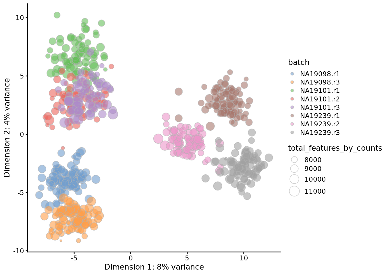
Figure 7.18: PCA plot of the tung data
scater allows one to identify principal components that correlate with
experimental and QC variables of interest (it ranks principle components by
\(R^2\) from a linear model regressing PC value against the variable of interest).
Let’s test whether some of the variables correlate with any of the PCs.
7.4.2.1 Top colData variables associated with PCs
The plot below shows, for each of the first 10 PCs, the variance explained by
the ten variables in colData(umi.qc) that are most strongly associated with
the PCs. [We will ignore the sample_id variable: it has a unique value for
each cell, so can explain all the variation for all PCs.]
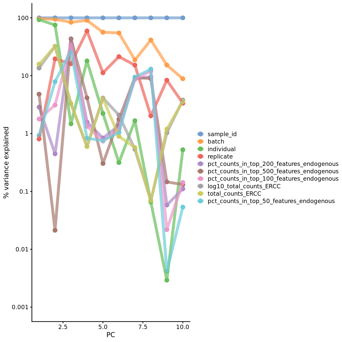
Figure 7.19: PC correlation with the number of detected genes
Indeed, we can see that PC1 can be almost completely explained by batch and
individual (of course batch is nested within individual). The total counts
from ERCC spike-ins also explains a substantial proportion of the variability in
PC1.
Although number of detected genes is not strongly correlated with the PCs here (after normalization), this is commonly the case and something to look out for. [You might like to replicate the plot above using raw logcounts values to see what happens without normalization]. This is a well-known issue in scRNA-seq and was described here.
7.4.3 Explanatory variables
scater can also compute the marginal \(R^2\) for each variable when fitting a
linear model regressing expression values for each gene against just that
variable, and display a density plot of the gene-wise marginal \(R^2\) values for
the variables.
plotExplanatoryVariables(
    umi.qc,
    exprs_values = "logcounts_raw",
    variables = c(
        "total_features_by_counts",
        "total_counts",
        "batch",
        "individual",
        "pct_counts_ERCC",
        "pct_counts_MT"
    )
)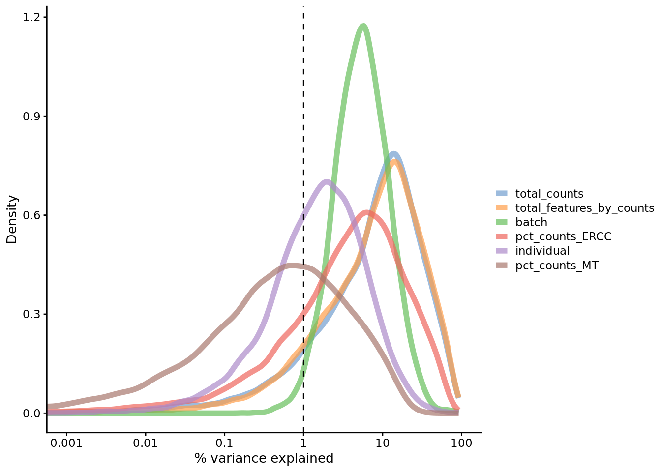
Figure 7.20: Explanatory variables
This analysis indicates that the number of detected genes (again) and also the
sequencing depth (total number of UMI counts per cell) have substantial
explanatory power for many genes, so these variables are good candidates for
conditioning out in a normalization step, or including in downstream statistical
models [cf. sctransform’s approach to normalization]. Expression of ERCCs also
appears to be an important explanatory variable and one notable feature of the
above plot is that batch explains more than individual. What does that tell us
about the technical and biological variability of the data?
7.4.4 Other confounders
In addition to correcting for batch, there are other factors that one may want to compensate for. As with batch correction, these adjustments require extrinsic information. One popular method is scLVM which allows you to identify and subtract the effect from processes such as cell-cycle or apoptosis.
In addition, protocols may differ in terms of their coverage of each transcript, their bias based on the average content of A/T nucleotides, or their ability to capture short transcripts. Ideally, we would like to compensate for all of these differences and biases.
7.4.5 Exercise
Perform the same analysis with read counts of the Blischak data. Use
tung/reads.rds file to load the reads SCESet object. Once you have finished
please compare your results to ours (next chapter).
7.4.6 sessionInfo()
## R version 3.6.0 (2019-04-26)
## Platform: x86_64-pc-linux-gnu (64-bit)
## Running under: Ubuntu 18.04.3 LTS
##
## Matrix products: default
## BLAS:   /usr/lib/x86_64-linux-gnu/blas/libblas.so.3.7.1
## LAPACK: /usr/lib/x86_64-linux-gnu/lapack/liblapack.so.3.7.1
##
## locale:
##  [1] LC_CTYPE=en_AU.UTF-8       LC_NUMERIC=C
##  [3] LC_TIME=en_AU.UTF-8        LC_COLLATE=en_AU.UTF-8
##  [5] LC_MONETARY=en_AU.UTF-8    LC_MESSAGES=en_AU.UTF-8
##  [7] LC_PAPER=en_AU.UTF-8       LC_NAME=C
##  [9] LC_ADDRESS=C               LC_TELEPHONE=C
## [11] LC_MEASUREMENT=en_AU.UTF-8 LC_IDENTIFICATION=C
##
## attached base packages:
## [1] parallel  stats4    stats     graphics  grDevices utils     datasets
## [8] methods   base
##
## other attached packages:
##  [1] scran_1.12.1                scater_1.12.2
##  [3] ggplot2_3.2.1               SingleCellExperiment_1.6.0
##  [5] SummarizedExperiment_1.14.1 DelayedArray_0.10.0
##  [7] BiocParallel_1.18.1         matrixStats_0.55.0
##  [9] Biobase_2.44.0              GenomicRanges_1.36.1
## [11] GenomeInfoDb_1.20.0         IRanges_2.18.3
## [13] S4Vectors_0.22.1            BiocGenerics_0.30.0
## [15] knitr_1.25
##
## loaded via a namespace (and not attached):
##  [1] locfit_1.5-9.1           Rcpp_1.0.2
##  [3] rsvd_1.0.2               lattice_0.20-38
##  [5] assertthat_0.2.1         digest_0.6.21
##  [7] R6_2.4.0                 dynamicTreeCut_1.63-1
##  [9] evaluate_0.14            highr_0.8
## [11] pillar_1.4.2             zlibbioc_1.30.0
## [13] rlang_0.4.0              lazyeval_0.2.2
## [15] irlba_2.3.3              Matrix_1.2-17
## [17] rmarkdown_1.15           labeling_0.3
## [19] BiocNeighbors_1.2.0      statmod_1.4.32
## [21] stringr_1.4.0            igraph_1.2.4.1
## [23] RCurl_1.95-4.12          munsell_0.5.0
## [25] compiler_3.6.0           vipor_0.4.5
## [27] BiocSingular_1.0.0       xfun_0.9
## [29] pkgconfig_2.0.3          ggbeeswarm_0.6.0
## [31] htmltools_0.3.6          tidyselect_0.2.5
## [33] tibble_2.1.3             gridExtra_2.3
## [35] GenomeInfoDbData_1.2.1   bookdown_0.13
## [37] edgeR_3.26.8             viridisLite_0.3.0
## [39] crayon_1.3.4             dplyr_0.8.3
## [41] withr_2.1.2              bitops_1.0-6
## [43] grid_3.6.0               gtable_0.3.0
## [45] magrittr_1.5             scales_1.0.0
## [47] dqrng_0.2.1              stringi_1.4.3
## [49] XVector_0.24.0           viridis_0.5.1
## [51] limma_3.40.6             DelayedMatrixStats_1.6.1
## [53] cowplot_1.0.0            tools_3.6.0
## [55] glue_1.3.1               beeswarm_0.2.3
## [57] purrr_0.3.2              yaml_2.2.0
## [59] colorspace_1.4-1
7.5 Identifying confounding factors (Reads)
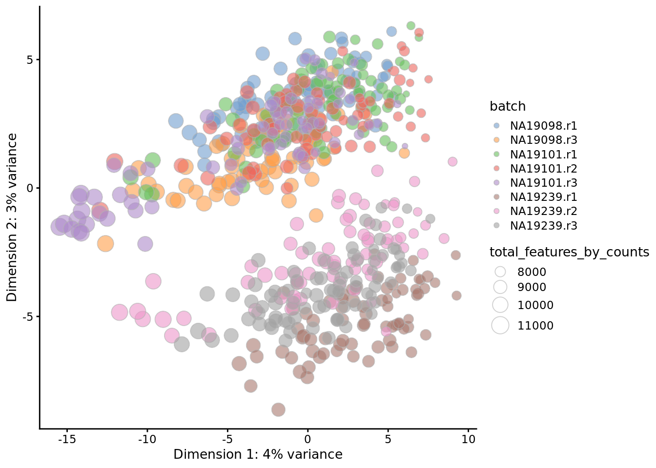
Figure 7.21: PCA plot of the tung data
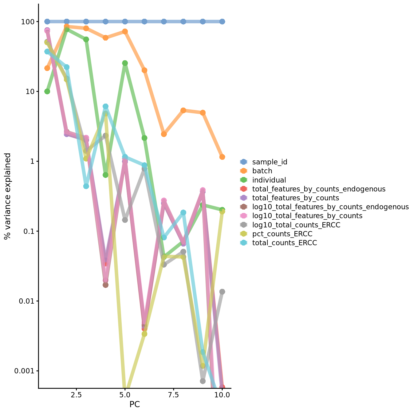
Figure 7.22: PC correlation with the number of detected genes
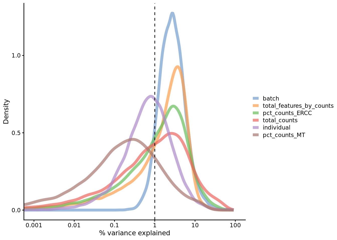
Figure 7.23: Explanatory variables
## R version 3.6.0 (2019-04-26)
## Platform: x86_64-pc-linux-gnu (64-bit)
## Running under: Ubuntu 18.04.3 LTS
##
## Matrix products: default
## BLAS:   /usr/lib/x86_64-linux-gnu/blas/libblas.so.3.7.1
## LAPACK: /usr/lib/x86_64-linux-gnu/lapack/liblapack.so.3.7.1
##
## locale:
##  [1] LC_CTYPE=en_AU.UTF-8       LC_NUMERIC=C
##  [3] LC_TIME=en_AU.UTF-8        LC_COLLATE=en_AU.UTF-8
##  [5] LC_MONETARY=en_AU.UTF-8    LC_MESSAGES=en_AU.UTF-8
##  [7] LC_PAPER=en_AU.UTF-8       LC_NAME=C
##  [9] LC_ADDRESS=C               LC_TELEPHONE=C
## [11] LC_MEASUREMENT=en_AU.UTF-8 LC_IDENTIFICATION=C
##
## attached base packages:
## [1] parallel  stats4    stats     graphics  grDevices utils     datasets
## [8] methods   base
##
## other attached packages:
##  [1] scran_1.12.1                scater_1.12.2
##  [3] ggplot2_3.2.1               SingleCellExperiment_1.6.0
##  [5] SummarizedExperiment_1.14.1 DelayedArray_0.10.0
##  [7] BiocParallel_1.18.1         matrixStats_0.55.0
##  [9] Biobase_2.44.0              GenomicRanges_1.36.1
## [11] GenomeInfoDb_1.20.0         IRanges_2.18.3
## [13] S4Vectors_0.22.1            BiocGenerics_0.30.0
##
## loaded via a namespace (and not attached):
##  [1] locfit_1.5-9.1           Rcpp_1.0.2
##  [3] rsvd_1.0.2               lattice_0.20-38
##  [5] assertthat_0.2.1         digest_0.6.21
##  [7] R6_2.4.0                 dynamicTreeCut_1.63-1
##  [9] evaluate_0.14            highr_0.8
## [11] pillar_1.4.2             zlibbioc_1.30.0
## [13] rlang_0.4.0              lazyeval_0.2.2
## [15] irlba_2.3.3              Matrix_1.2-17
## [17] rmarkdown_1.15           labeling_0.3
## [19] BiocNeighbors_1.2.0      statmod_1.4.32
## [21] stringr_1.4.0            igraph_1.2.4.1
## [23] RCurl_1.95-4.12          munsell_0.5.0
## [25] compiler_3.6.0           vipor_0.4.5
## [27] BiocSingular_1.0.0       xfun_0.9
## [29] pkgconfig_2.0.3          ggbeeswarm_0.6.0
## [31] htmltools_0.3.6          tidyselect_0.2.5
## [33] tibble_2.1.3             gridExtra_2.3
## [35] GenomeInfoDbData_1.2.1   bookdown_0.13
## [37] edgeR_3.26.8             viridisLite_0.3.0
## [39] crayon_1.3.4             dplyr_0.8.3
## [41] withr_2.1.2              bitops_1.0-6
## [43] grid_3.6.0               gtable_0.3.0
## [45] magrittr_1.5             scales_1.0.0
## [47] dqrng_0.2.1              stringi_1.4.3
## [49] XVector_0.24.0           viridis_0.5.1
## [51] limma_3.40.6             DelayedMatrixStats_1.6.1
## [53] cowplot_1.0.0            tools_3.6.0
## [55] glue_1.3.1               beeswarm_0.2.3
## [57] purrr_0.3.2              yaml_2.2.0
## [59] colorspace_1.4-1         knitr_1.25
7.6 Batch effects
7.6.1 Introduction
In the previous chapter we normalized for library size, effectively removing it as a confounder. Now we will consider removing other less well defined confounders from our data. Technical confounders (aka batch effects) can arise from difference in reagents, isolation methods, the lab/experimenter who performed the experiment, even which day/time the experiment was performed. Accounting for technical confounders, and batch effects particularly, is a large topic that also involves principles of experimental design. Here we address approaches that can be taken to account for confounders when the experimental design is appropriate.
Fundamentally, accounting for technical confounders involves identifying and, ideally, removing sources of variation in the expression data that are not related to (i.e. are confounding) the biological signal of interest. Various approaches exist, some of which use spike-in or housekeeping genes, and some of which use endogenous genes.
7.6.1.1 Advantages and disadvantages of using spike-ins to remove confounders
The use of spike-ins as control genes is conceptually appealing, since (ideally) the same amount of ERCC (or other) spike-in would be added to each cell in our experiment. In principle, all the variability we observe for these ``genes’’ is due to technical noise; whereas endogenous genes are affected by both technical noise and biological variability. Technical noise can be removed by fitting a model to the spike-ins and “substracting” this from the endogenous genes. There are several methods available based on this premise (eg. BASiCS, scLVM, RUVg); each using different noise models and different fitting procedures. Alternatively, one can identify genes which exhibit significant variation beyond technical noise (eg. Distance to median, Highly variable genes).
Unfortunately, there are major issues with the use of spike-ins for normalisation that limit their utility in practice. Perhaps surprisingly, their variability can, for various reasons, actually be higher than that of endogenous genes. One key reason for the difficulty of their use in practice is the need to pipette miniscule volumes of spike-in solution into The most popular set of spike-ins, namely ERCCs, are derived from bacterial sequences, which raises concerns that their base content and structure diverges to far from gene structure in other biological systems of interest (e.g. mammalian genes) to be reliable for normalisation. Even in the best-case scenarios, spike-ins are limited to use on plate-based platforms; they are fundamentally incompatible with droplet-based platforms.
Given the issues with using spike-ins, better results can often be obtained by using endogenous genes instead. Given their limited availability, normalisation methods based only on endogenous genes needed to be developed and we consider them generally preferable, even for platforms where spike-ins may be used. Where we have a large number of endogenous genes that, on average, do not vary systematically between cells and where we expect technical effects to affect a large number of genes (a very common and reasonable assumption), then such methods (for example, the RUVs method) can perform well.
We explore both general approaches below.
library(scRNA.seq.funcs)
library(RUVSeq)
library(scater)
library(SingleCellExperiment)
library(scran)
library(kBET)
library(sva) # Combat
library(edgeR)
library(harmony)
set.seed(1234567)
options(stringsAsFactors = FALSE)
umi <- readRDS("data/tung/umi.rds")
umi.qc <- umi[rowData(umi)$use, colData(umi)$use]
endog_genes <- !rowData(umi.qc)$is_feature_control
erccs <- rowData(umi.qc)$is_feature_control
## Apply scran sum factor normalization
qclust <- quickCluster(umi.qc, min.size = 30, use.ranks = FALSE)
umi.qc <- computeSumFactors(umi.qc, sizes = 15, clusters = qclust)
umi.qc <- normalize(umi.qc)
7.6.2 Linear models
Linear models offer a relatively simple approach to accounting for batch effects
and confounders. A linear model can correct for batches while preserving
biological effects if you have a balanced design. In a confounded/replicate
design biological effects will not be fit/preserved. We could remove batch
effects from each individual separately in order to preserve biological (and
technical) variance between individuals (we will apply a similar with
mnnCorrect, below).
Depending on how we have pre-processed our scRNA-seq data or what modelling assumptions we are willing to make, we may choose to use normal (Gaussian) linear models (i.e. assuming a normal distribution for noise) or generalized linear models (GLM), where we can use any distribution from the exponential family. Given that we obtain highly-variable count data from scRNA-seq assays, the obvious choice for a GLM is to use the negative binomial distribution, which has proven highly successful in the analysis of bulk RNA-seq data.
For demonstration purposes here we will naively correct all confounded batch effects.
7.6.2.1 Gaussian (normal) linear models
The limma
package in Bioconductor offers a convenient and efficient means to fit a linear
model (with the same design matrix) to a dataset with a large number of features
(i.e. genes) (Ritchie et al. 2015). An added advantage of limma is its ability to
apply empirical Bayes squeezing of variance estimate to improve inference.
Provided we are satisfied making the assumption of a Gaussian distribution for
residuals (this may be reasonable for normalized log-counts in many cases; but
it may not be—debate continues in the literature), then we can apply limma
to regress out (known) unwanted sources of variation as follows.
## fit a model just accounting for batch
lm_design_batch <- model.matrix(~0 + batch, data = colData(umi.qc))
fit_lm_batch <- lmFit(logcounts(umi.qc), lm_design_batch)
resids_lm_batch <- residuals(fit_lm_batch, logcounts(umi.qc))
assay(umi.qc, "lm_batch") <- resids_lm_batch

reducedDim(umi.qc, "PCA_lm_batch") <- reducedDim(
  runPCA(umi.qc[endog_genes, ], exprs_values = "lm_batch"), "PCA")

plotReducedDim(umi.qc, use_dimred = "PCA_lm_batch",
        colour_by = "batch",
        size_by = "total_features_by_counts",
        shape_by = "individual"
        ) +
  ggtitle("LM - regress out batch")
Two problems are immediately apparent with the approach above. First, batch is nested within individual, so simply regressing out batch as we have done above also regresses out differences between individuals that we would like to preserve. Second, we observe that the first principal component seems to separate cells by number of genes (features) expressed, which is undesirable.
We can address these concerns by correcting for batch within each individual separately, and also fitting the proportion of genes expressed per cell as a covariate. [NB: to preserve overall differences in expression levels between individuals we will need to apply a slight hack to the LM fit results (setting the intercept coefficient to zero).]
Exercise 2
Perform LM correction for each individual separately. Store the final corrected
matrix in the lm_batch_indi slot.
## define cellular detection rate (cdr), i.e. proportion of genes expressed in each cell
umi.qc$cdr <- umi.qc$total_features_by_counts_endogenous / nrow(umi.qc)
## fit a model just accounting for batch by individual
lm_design_batch1 <- model.matrix(~batch + cdr,
                                 data = colData(umi.qc)[umi.qc$individual == "na19098",])
fit_indi1 <- lmfit(logcounts(umi.qc)[, umi.qc$individual == "na19098"], lm_design_batch1)
fit_indi1$coefficients[,1] <- 0 ## replace intercept with 0 to preserve reference batch
resids_lm_batch1 <- residuals(fit_indi1, logcounts(umi.qc)[, umi.qc$individual == "na19098"])

lm_design_batch2 <- model.matrix(~batch + cdr,
                                 data = colData(umi.qc)[umi.qc$individual == "na19101",])
fit_indi2 <- lmfit(logcounts(umi.qc)[, umi.qc$individual == "na19101"], lm_design_batch2)
fit_indi2$coefficients[,1] <- 0 ## replace intercept with 0 to preserve reference batch
resids_lm_batch2 <- residuals(fit_indi2, logcounts(umi.qc)[, umi.qc$individual == "na19101"])

lm_design_batch3 <- model.matrix(~batch + cdr,
                                 data = colData(umi.qc)[umi.qc$individual == "na19239",])
fit_indi3 <- lmfit(logcounts(umi.qc)[, umi.qc$individual == "na19239"], lm_design_batch3)
fit_indi3$coefficients[,1] <- 0 ## replace intercept with 0 to preserve reference batch
resids_lm_batch3 <- residuals(fit_indi3, logcounts(umi.qc)[, umi.qc$individual == "na19239"])

identical(colnames(umi.qc), colnames(cbind(resids_lm_batch1, resids_lm_batch2, resids_lm_batch3)))
assay(umi.qc, "lm_batch_indi") <- cbind(resids_lm_batch1, resids_lm_batch2, resids_lm_batch3)

reduceddim(umi.qc, "pca_lm_batch_indi") <- reduceddim(
  runpca(umi.qc[endog_genes, ], exprs_values = "lm_batch_indi"), "pca")

plotreduceddim(umi.qc, use_dimred = "pca_lm_batch_indi",
        colour_by = "batch",
        size_by = "total_features_by_counts",
        shape_by = "individual"
        ) +
  ggtitle("lm - regress out batch within individuals separately")
What do you think of the results of this approach?
7.6.2.2 Negative binomial generalized linear models
Advanced exercise
Can you use the edgeR package to use a negative binomial generalized linear
model to regress out batch effects?
Hint: follow a similar approach to that taken in the limma example above.
You will need to use the DGEList(), estimateDisp(), and glmQLFit()
functions.
7.6.3 sctransform
The sctransform approach to using Pearson residuals from an regularized
negative binomial generalized linear model was introduced above. Here we
demonstrate how to apply this method.
Note that (due to what looks like a bug in this version of sctransform) we
need to convert the UMI count matrix to a sparse format to apply sctransform.
These sctransform results will face the problem mentioned above of batch being
nested within individual, which means that we cannot directly remove batch
effects without removing differences between individuals. However, here we will
demonstrate how you would try to remove batch effects with sctransform for a
kinder experimental design.
umi_sparse <- as(counts(umi.qc), "dgCMatrix")
### Genes expressed in at least 5 cells will be kept
sctnorm_data <- sctransform::vst(umi = umi_sparse, min_cells = 1,
                                 cell_attr = as.data.frame(colData(umi.qc)),
                                 latent_var = c("log10_total_counts_endogenous", "batch"))
## Pearson residuals, or deviance residuals
sctnorm_data$model_str
assay(umi.qc, "sctrans_norm") <- sctnorm_data$y
Let us look at the NB GLM model parameters estimated by sctransform.
#sce$log10_total_counts
##       Matrix of estimated model parameters per gene (theta and regression coefficients)
sctransform::plot_model_pars(sctnorm_data)![]()
Do these parameters and the regularization look sensible to you? Any concerns?
reducedDim(umi.qc, "PCA_sctrans_norm") <- reducedDim(
  runPCA(umi.qc[endog_genes, ], exprs_values = "sctrans_norm")
)
plotReducedDim(
  umi.qc,
  use_dimred = "PCA_sctrans_norm",
  colour_by = "batch",
  size_by = "total_features_by_counts",
  shape_by = "individual"
) + ggtitle("PCA plot: sctransform normalization") 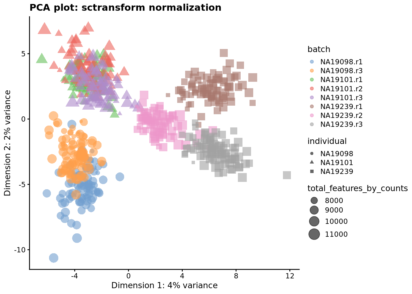
Figure 7.7: PCA plot of the tung data after sctransform normalisation (Pearson residuals).
Q: What’s happened here? Was that expected? Any other comments?
7.6.4 Remove Unwanted Variation
Factors contributing to technical noise frequently appear as “batch effects” where cells processed on different days or by different technicians systematically vary from one another. Removing technical noise and correcting for batch effects can frequently be performed using the same tool or slight variants on it. We will be considering the Remove Unwanted Variation (RUVSeq). Briefly, RUVSeq works as follows. For \(n\) samples and \(J\) genes, consider the following generalized linear model (GLM), where the RNA-Seq read counts are regressed on both the known covariates of interest and unknown factors of unwanted variation: \[\log E[Y|W,X,O] = W\alpha + X\beta + O\] Here, \(Y\) is the \(n \times J\) matrix of observed gene-level read counts, \(W\) is an \(n \times k\) matrix corresponding to the factors of “unwanted variation” and \(O\) is an \(n \times J\) matrix of offsets that can either be set to zero or estimated with some other normalization procedure (such as upper-quartile normalization). The simultaneous estimation of \(W\), \(\alpha\), \(\beta\), and \(k\) is infeasible. For a given \(k\), instead the following three approaches to estimate the factors of unwanted variation \(W\) are used:
- RUVg uses negative control genes (e.g. ERCCs), assumed to have constant expression across samples;
- RUVs uses centered (technical) replicate/negative control samples for which the covariates of interest are constant;
- RUVr uses residuals, e.g., from a first-pass GLM regression of the counts on the covariates of interest.
We will concentrate on the first two approaches.
7.6.4.1 RUVg
To use RUVg we will use ERCCs as negative control genes to anchor the estimation of factors representing unwanted variation. RUVg operates on the raw count data. We adjust the output normalized counts from RUVg so that they represent normalized counts-per-million and then apply a log2 transformation. We run RUVg twice, with \(k=1\) and \(k=10\) so that we can compare the effect of estimating different number of hidden factors to capture unwanted variation in the data.
ruvg <- RUVg(counts(umi.qc), erccs, k = 1)
assay(umi.qc, "ruvg1") <- log2(
    t(t(ruvg$normalizedCounts) / colSums(ruvg$normalizedCounts) * 1e6) + 1
)
ruvg <- RUVg(counts(umi.qc), erccs, k = 10)
assay(umi.qc, "ruvg10") <- log2(
    t(t(ruvg$normalizedCounts) / colSums(ruvg$normalizedCounts) * 1e6) + 1
)
When we assess the effectiveness of various batch correction methods below, you can discuss whether or not you think using ERCCs as negative control genes for a method like RUVg is advisable (in this dataset and in general).
7.6.4.2 RUVs
In this application of RUVs we treat the individuals as replicates for which the covariates of interest are constant.
As above, we adjust the output normalized counts from RUVs so that they represent normalized counts-per-million and then apply a log2 transformation. Again, we run the method with \(k=1\) and \(k=10\) so that we can compare the effect of estimating different number of hidden factors.
scIdx <- matrix(-1, ncol = max(table(umi.qc$individual)), nrow = 3)
tmp <- which(umi.qc$individual == "NA19098")
scIdx[1, 1:length(tmp)] <- tmp
tmp <- which(umi.qc$individual == "NA19101")
scIdx[2, 1:length(tmp)] <- tmp
tmp <- which(umi.qc$individual == "NA19239")
scIdx[3, 1:length(tmp)] <- tmp
cIdx <- rownames(umi.qc)
ruvs <- RUVs(counts(umi.qc), cIdx, k = 1, scIdx = scIdx, isLog = FALSE)
assay(umi.qc, "ruvs1") <- log2(
    t(t(ruvs$normalizedCounts) / colSums(ruvs$normalizedCounts) * 1e6) + 1
)
ruvs <- RUVs(counts(umi.qc), cIdx, k = 10, scIdx = scIdx, isLog = FALSE)
assay(umi.qc, "ruvs10") <- log2(
    t(t(ruvs$normalizedCounts) / colSums(ruvs$normalizedCounts) * 1e6) + 1
)
7.6.5 Combat
If you have an experiment with a balanced design, Combat can be used to
eliminate batch effects while preserving biological effects by specifying the
biological effects using the mod parameter. However the Tung data contains
multiple experimental replicates rather than a balanced design so using mod1
to preserve biological variability will result in an error.
combat_data <- logcounts(umi.qc)
mod_data <- as.data.frame(t(combat_data))
# Basic batch removal
mod0 <- model.matrix(~ 1, data = mod_data)
# Preserve biological variability
mod1 <- model.matrix(~ umi.qc$individual, data = mod_data)
# adjust for total genes detected
mod2 <- model.matrix(~ umi.qc$total_features_by_counts, data = mod_data)
assay(umi.qc, "combat") <- ComBat(
    dat = t(mod_data),
    batch = factor(umi.qc$batch),
    mod = mod0,
    par.prior = TRUE,
    prior.plots = FALSE
)
## Standardizing Data across genesExercise 1
Perform ComBat correction accounting for total features as a co-variate. Store the corrected matrix in the combat_tf slot.
7.6.6 mnnCorrect
mnnCorrect (Haghverdi et al. 2017) assumes that each batch shares at least one
biological condition with each other batch. Thus it works well for a variety of
balanced experimental designs. However, the Tung data contains multiple
replicates for each invidividual rather than balanced batches, thus we will
normalize each individual separately. Note that this will remove batch effects
between batches within the same individual but not the batch effects between
batches in different individuals, due to the confounded experimental design.
Thus we will merge a replicate from each individual to form three batches.
do_mnn <- function(data.qc) {
    batch1 <- logcounts(data.qc[, data.qc$replicate == "r1"])
    batch2 <- logcounts(data.qc[, data.qc$replicate == "r2"])
    batch3 <- logcounts(data.qc[, data.qc$replicate == "r3"])

    if (ncol(batch2) > 0) {
        x <- batchelor::mnnCorrect(
          batch1, batch2, batch3,
          k = 20,
          sigma = 0.1,
          cos.norm.in = TRUE,
          svd.dim = 2
        )
        return(x)
    } else {
        x <- batchelor::mnnCorrect(
          batch1, batch3,
          k = 20,
          sigma = 0.1,
          cos.norm.in = TRUE,
          svd.dim = 2
        )
        return(x)
    }
}

indi1 <- do_mnn(umi.qc[, umi.qc$individual == "NA19098"])
indi2 <- do_mnn(umi.qc[, umi.qc$individual == "NA19101"])
indi3 <- do_mnn(umi.qc[, umi.qc$individual == "NA19239"])

identical(colnames(umi.qc), colnames(cbind(indi1, indi2, indi3)))
## [1] TRUEassay(umi.qc, "mnn") <- assay(cbind(indi1, indi2, indi3), "corrected")
# For a balanced design:
#assay(umi.qc, "mnn") <- mnnCorrect(
# list(B1 = logcounts(batch1), B2 = logcounts(batch2), B3 = logcounts(batch3)),
# k = 20,
# sigma = 0.1,
# cos.norm = TRUE,
# svd.dim = 2
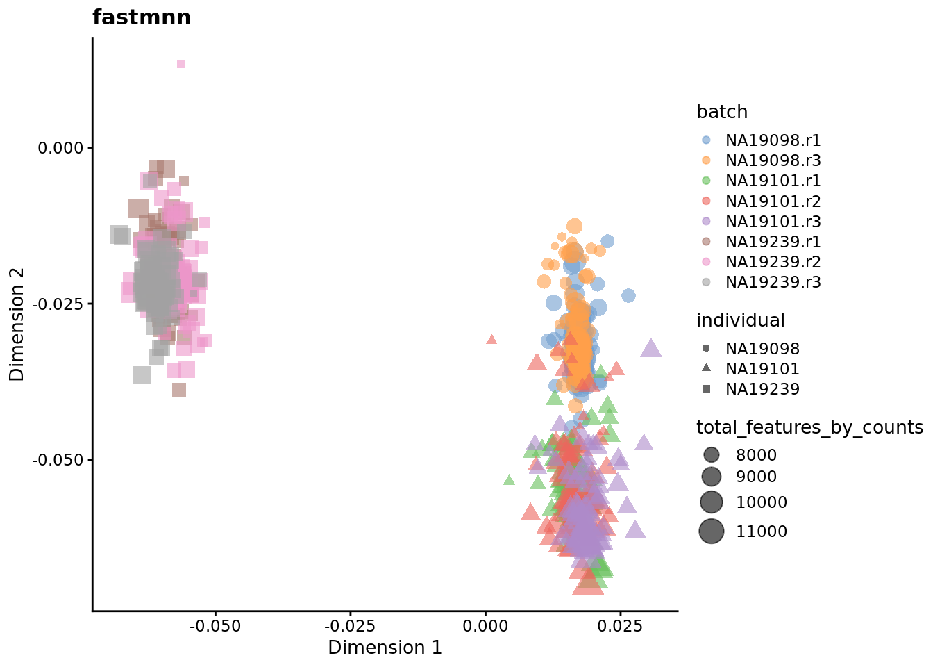
#)The latest version of the
batchelor
package has a new fastMNN() method. The fastMNN() function performs a
principal components (PCA). MNN identification and correction is preformed on
this low-dimensional representation of the data, an approach that offers some
advantages in speed and denoising. The function returns a SingleCellExperiment
object containing a matrix of corrected PC scores, which can be used directly
for downstream analyses like clustering and visualization. [NB: fastMNN may
actually be slower on small datasets like that considered here.]
indi1 <- batchelor::fastMNN(
umi.qc[, umi.qc$individual == "NA19098"],
batch = umi.qc[, umi.qc$individual == "NA19098"]$replicate)
indi2 <- batchelor::fastMNN(
umi.qc[, umi.qc$individual == "NA19101"],
batch = umi.qc[, umi.qc$individual == "NA19101"]$replicate)
indi3 <- batchelor::fastMNN(
umi.qc[, umi.qc$individual == "NA19239"],
batch = umi.qc[, umi.qc$individual == "NA19239"]$replicate)
identical(colnames(umi.qc),
colnames(cbind(assay(indi1, "reconstructed"),
assay(indi2, "reconstructed"),
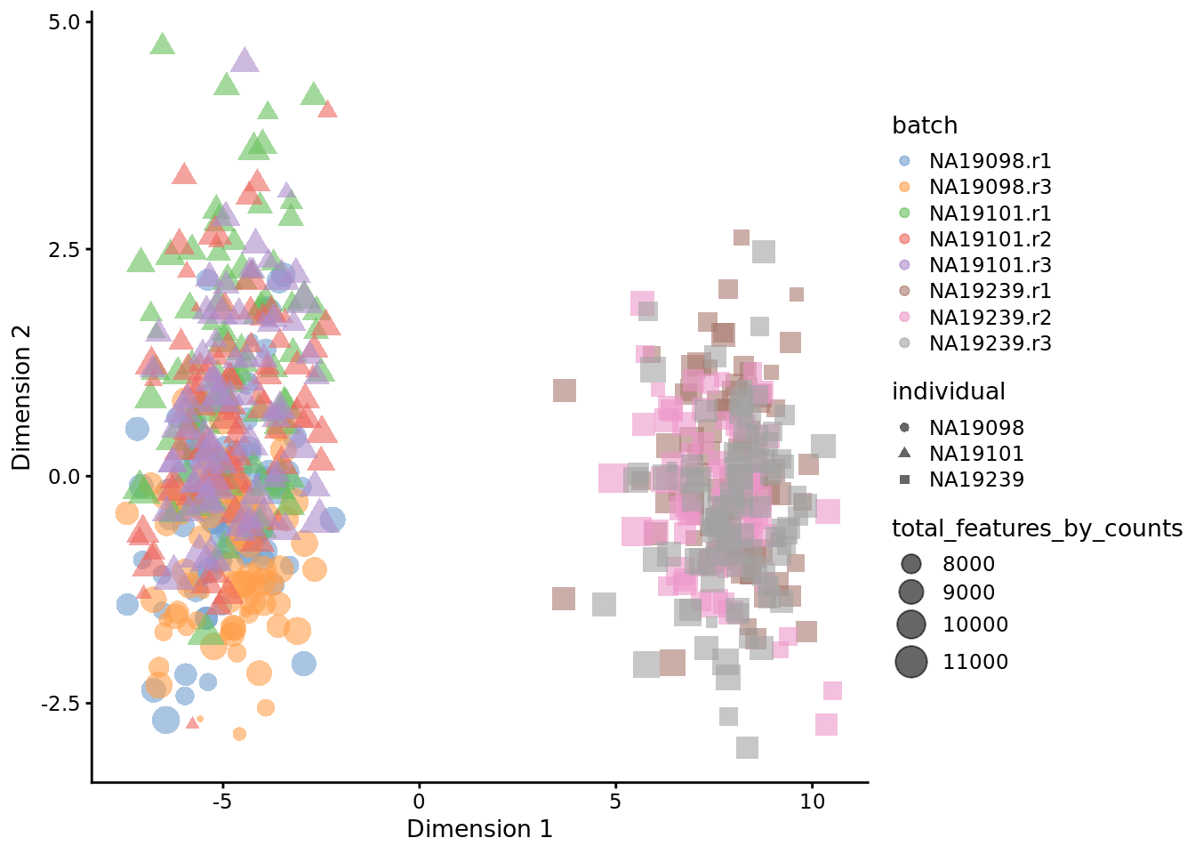
assay(indi3, "reconstructed")))) ## [1] TRUEfastmnn <- cbind(assay(indi1, "reconstructed"),
assay(indi2, "reconstructed"),
assay(indi3, "reconstructed"))
identical(rownames(umi.qc), rownames(fastmnn))## [1] FALSE## fastMNN() drops 66 genes, so we cannot immediately add the reconstructed expression matrix to assays() in umi.qc
## But we can run PCA on the reconstructed data from fastMNN() and add that to the reducedDim slot of our SCE object
fastmnn_pca <- runPCA(fastmnn, rank=2)
reducedDim(umi.qc, "fastmnn") <- fastmnn_pca$rotationFor further details, please consult the batchelor package documentation and
vignette.
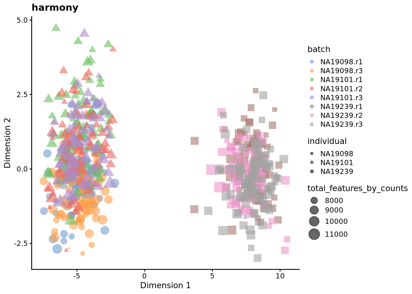
7.6.7 Harmony
Harmony [Korsunsky2018fast] is a newer batch correction method, which is
designed to operate on PC space. The algorithm proceeds to iteratively cluster
the cells, with the objective function formulated to promote cells from multiple
datasets within each cluster. Once a clustering is obtained, the positions of
the centroids of each dataset are obtained on a per-cluster basis and the
coordinates are corrected. This procedure is iterated until convergence. Harmony
comes with a theta parameter that controls the degree of batch correction
(higher values lead to more dataset integration), and can account for multiple
experimental and biological factors on input.
Seeing how the end result of Harmony is an altered dimensional reduction space created on the basis of PCA, we plot the obtained manifold here and exclude it from the rest of the follow-ups in the section.
umi.qc.endog <- umi.qc[endog_genes,]
umi.qc.endog <- runPCA(umi.qc.endog, exprs_values = 'logcounts', ncomponents = 20)
pca <- as.matrix(reducedDim(umi.qc.endog, "PCA"))
harmony_emb <- HarmonyMatrix(pca, umi.qc.endog$batch, theta=2, do_pca=FALSE)
reducedDim(umi.qc.endog, "harmony") <- harmony_emb

plotReducedDim(
    umi.qc.endog,
    use_dimred = 'harmony',
    colour_by = "batch",
    size_by = "total_features_by_counts",
    shape_by = "individual"
)
7.6.8 How to evaluate and compare batch correction
A key question when considering the different methods for removing confounders is how to quantitatively determine which one is the most effective. The main reason why comparisons are challenging is because it is often difficult to know what corresponds to technical counfounders and what is interesting biological variability. Here, we consider three different metrics which are all reasonable based on our knowledge of the experimental design. Depending on the biological question that you wish to address, it is important to choose a metric that allows you to evaluate the confounders that are likely to be the biggest concern for the given situation.
7.6.8.1 Effectiveness 1
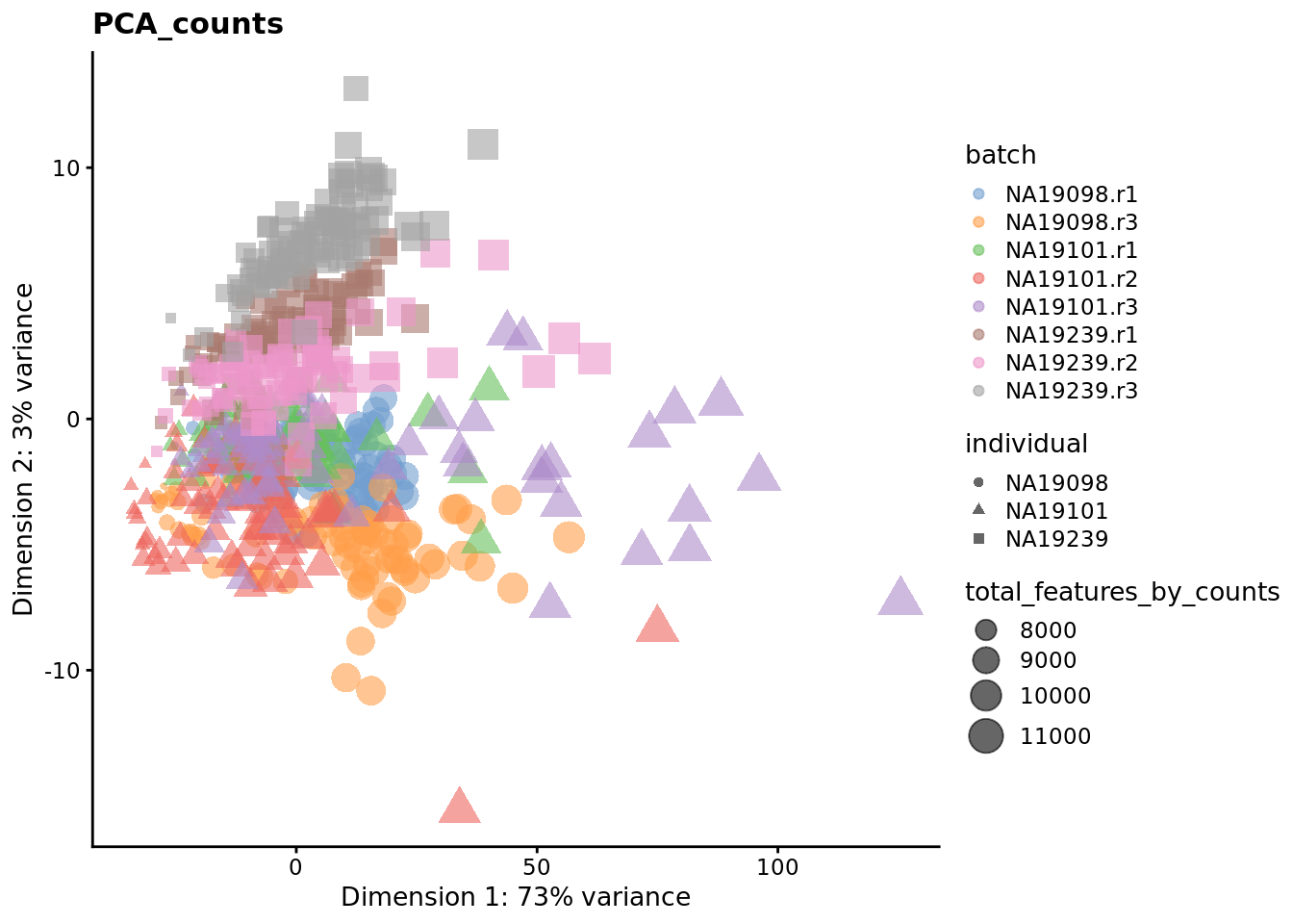
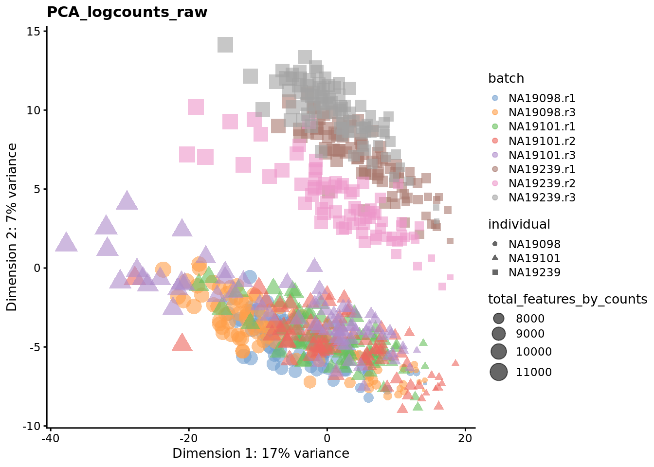
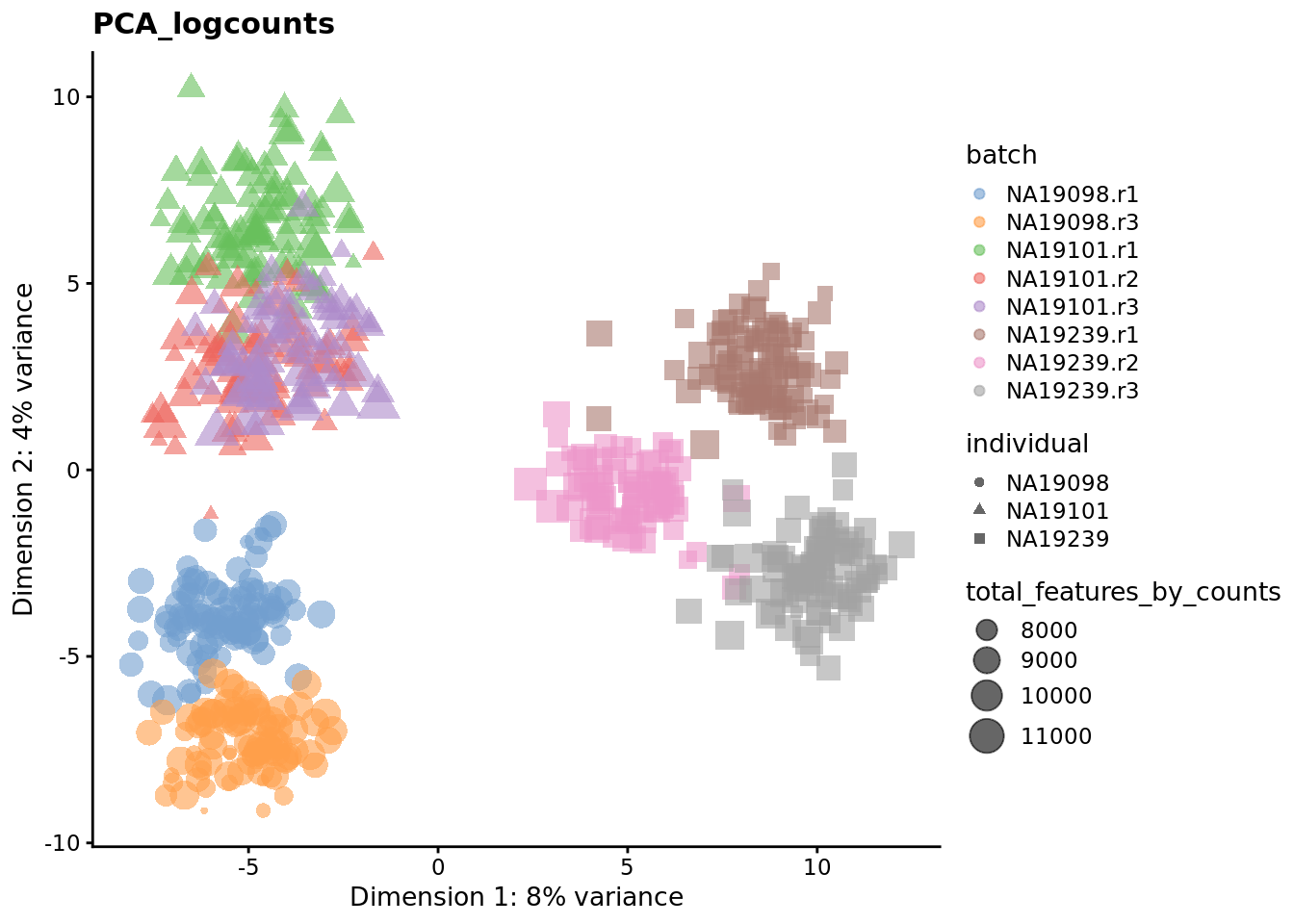
We evaluate the effectiveness of the normalization by inspecting the PCA plot where colour corresponds the technical replicates and shape corresponds to different biological samples (individuals). Separation of biological samples and interspersed batches indicates that technical variation has been removed. We always use log2-cpm normalized data to match the assumptions of PCA.
for (nm in assayNames(umi.qc)) {
  cat(nm, " \n")
  tmp <- runPCA(
    umi.qc[endog_genes, ],
    exprs_values = nm
  )
  reducedDim(umi.qc, paste0("PCA_", nm)) <- reducedDim(tmp, "PCA")
}
## counts
## logcounts_raw
## logcounts
## sctrans_norm
## ruvg1
## ruvg10
## ruvs1
## ruvs10
## combat
## mnnfor (nm in reducedDimNames(umi.qc)) {
print(
plotReducedDim(
umi.qc,
use_dimred = nm,
colour_by = "batch",
size_by = "total_features_by_counts",
shape_by = "individual"
) +
ggtitle(nm)
)
}
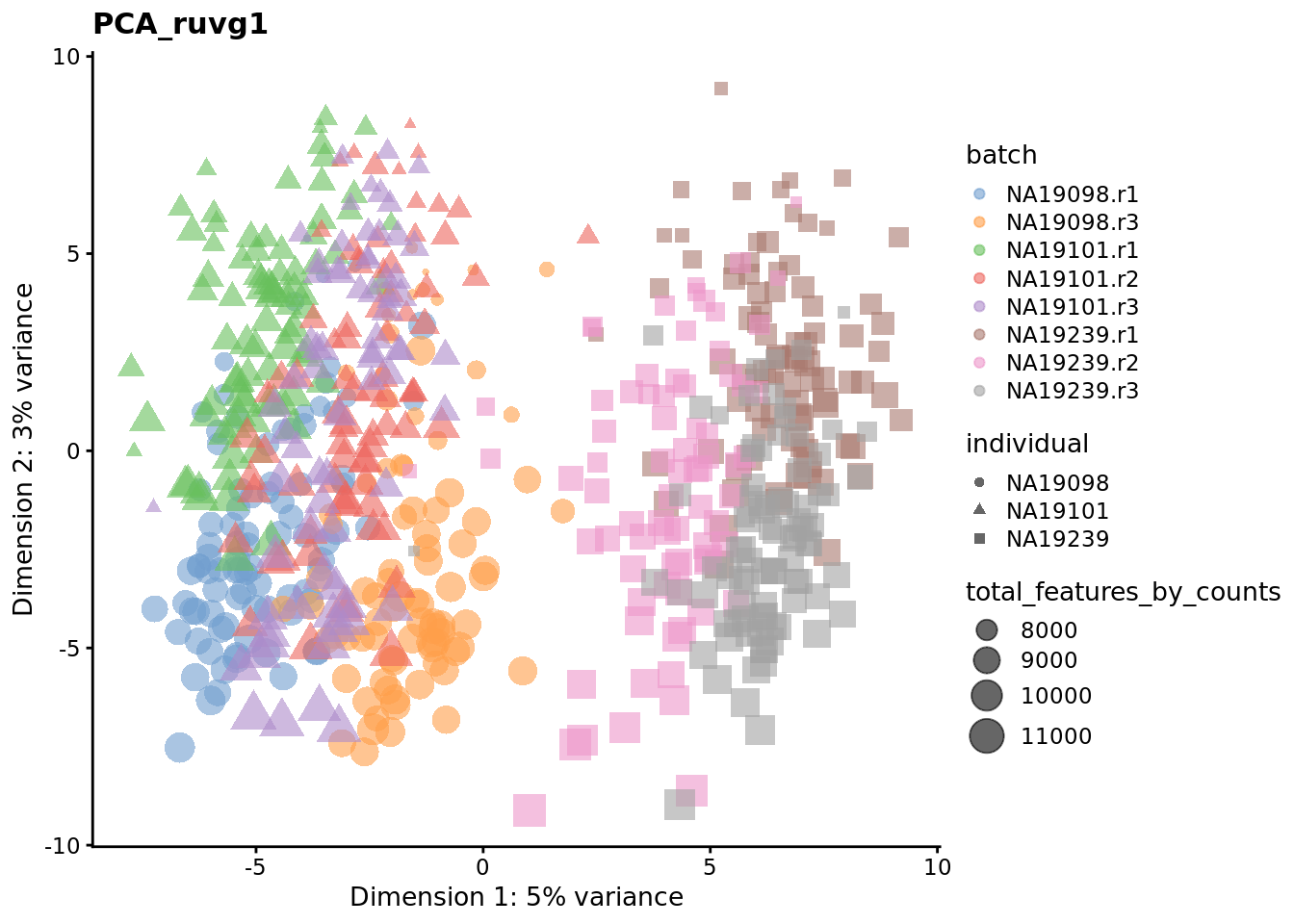
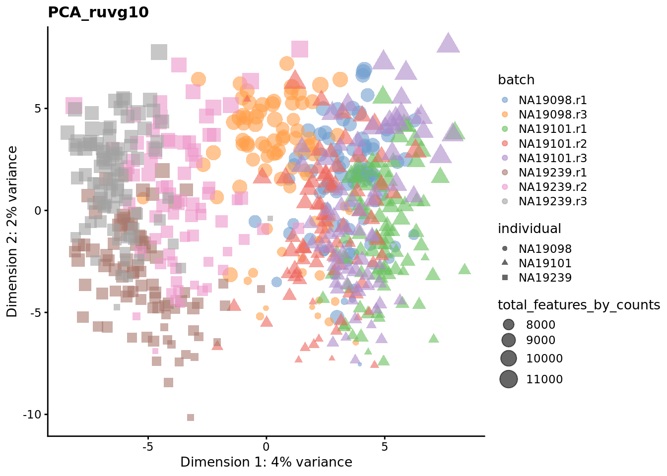
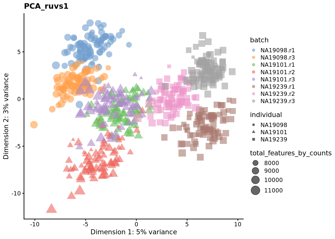
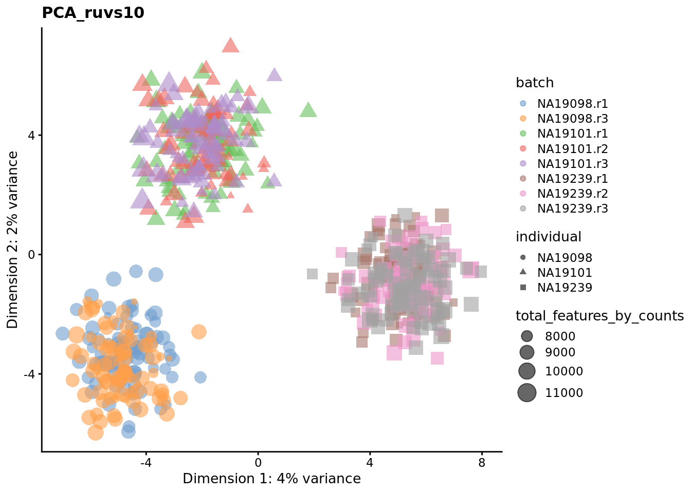
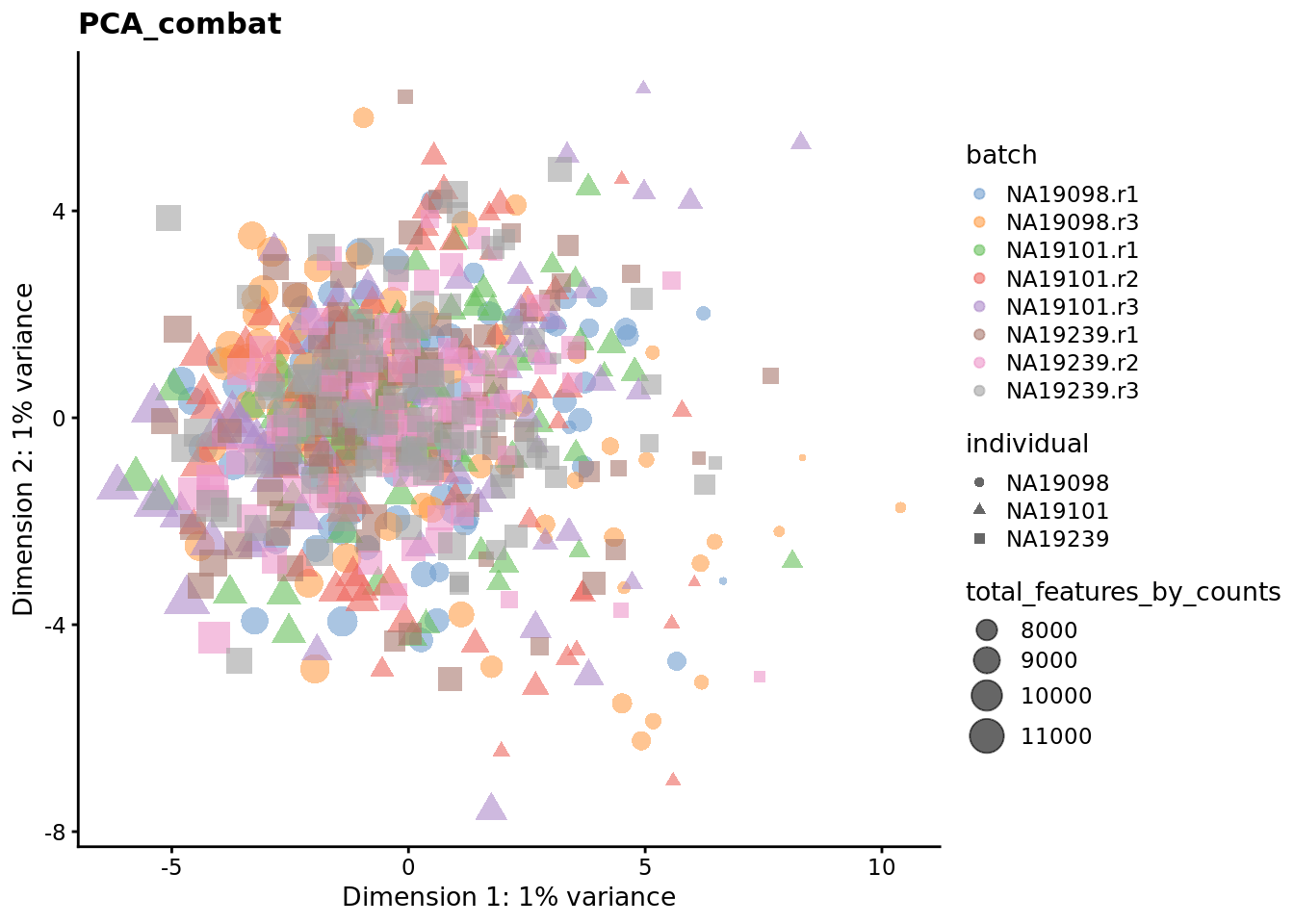
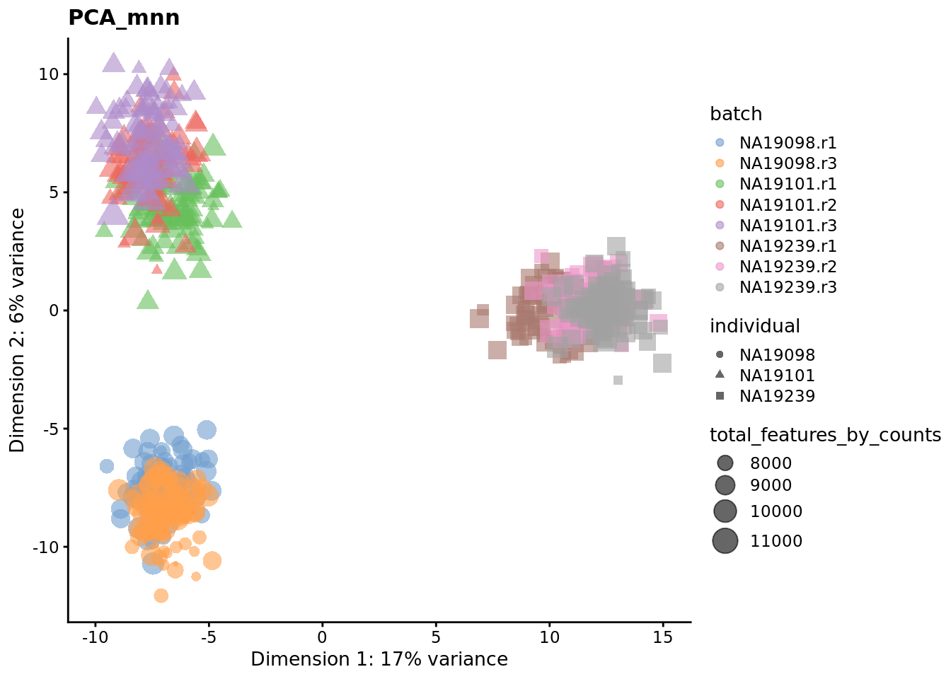
Exercise 3
Consider different k’s for RUV normalizations. Which gives the best results?
7.6.8.2 Effectiveness 2
We can also examine the effectiveness of correction using the relative log expression (RLE) across cells to confirm technical noise has been removed from the dataset. Note RLE only evaluates whether the number of genes higher and lower than average are equal for each cell - i.e. systemic technical effects. Random technical noise between batches may not be detected by RLE.
res <- list()
for(n in assayNames(umi.qc)) {
    res[[n]] <- suppressWarnings(calc_cell_RLE(assay(umi.qc, n), erccs))
}
par(mar=c(6,4,1,1))
boxplot(res, las=2)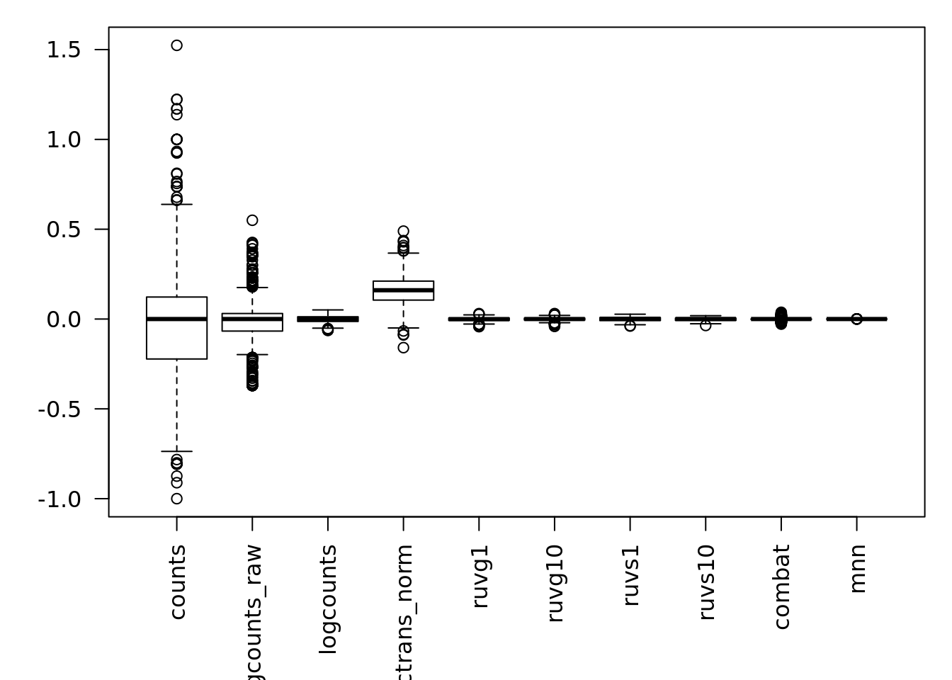
7.6.8.3 Effectiveness 3
Another method to check the efficacy of batch-effect correction is to consider the intermingling of points from different batches in local subsamples of the data. If there are no batch-effects then proportion of cells from each batch in any local region should be equal to the global proportion of cells in each batch.
kBET (Buttner et al. 2017) takes kNN networks around random cells and tests the
number of cells from each batch against a binomial distribution. The rejection
rate of these tests indicates the severity of batch-effects still present in the
data (high rejection rate = strong batch effects). kBET assumes each batch
contains the same complement of biological groups, thus it can only be applied
to the entire dataset if a perfectly balanced design has been used. However,
kBET can also be applied to replicate-data if it is applied to each biological
group separately. In the case of the Tung data, we will apply kBET to each
individual independently to check for residual batch effects. However, this
method will not identify residual batch-effects which are confounded with
biological conditions. In addition, kBET does not determine if biological
signal has been preserved.
compare_kBET_results <- function(sce){
    indiv <- unique(sce$individual)
    norms <- assayNames(sce) # Get all normalizations
    results <- list()
    for (i in indiv){
        for (j in norms){
            tmp <- kBET(
                df = t(assay(sce[,sce$individual== i], j)),
                batch = sce$batch[sce$individual==i],
                heuristic = TRUE,
                verbose = FALSE,
                addTest = FALSE,
                plot = FALSE)
            results[[i]][[j]] <- tmp$summary$kBET.observed[1]
        }
    }
    return(as.data.frame(results))
}

eff_debatching <- compare_kBET_results(umi.qc)require("reshape2")
require("RColorBrewer")
# Plot results
dod <- melt(as.matrix(eff_debatching), value.name = "kBET")
colnames(dod)[1:2] <- c("Normalisation", "Individual")
colorset <- c('gray', brewer.pal(n = 9, "Oranges"))
ggplot(dod, aes(Normalisation, Individual, fill=kBET)) +
geom_tile() +
scale_fill_gradient2(
na.value = "gray",
low = colorset[2],
mid=colorset[6],
high = colorset[10],
midpoint = 0.5, limit = c(0,1)) +
scale_x_discrete(expand = c(0, 0)) +
scale_y_discrete(expand = c(0, 0)) +
theme(
axis.text.x = element_text(
angle = 45,
vjust = 1,
size = 12,
hjust = 1
)
) +
ggtitle("Effect of batch regression methods per individual")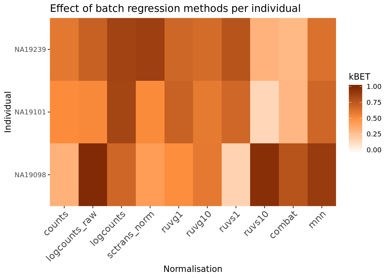
Exercise 4
Why do the raw counts appear to have little batch effects?
7.6.9 Big Exercise
Perform the same analysis with read counts of the tung data. Use
tung/reads.rds file to load the reads SCE object. Once you have finished
please compare your results to ours (next chapter). Additionally, experiment
with other combinations of normalizations and compare the results.
7.6.10 sessionInfo()
## R version 3.6.0 (2019-04-26)
## Platform: x86_64-pc-linux-gnu (64-bit)
## Running under: Ubuntu 18.04.3 LTS
##
## Matrix products: default
## BLAS:   /usr/lib/x86_64-linux-gnu/blas/libblas.so.3.7.1
## LAPACK: /usr/lib/x86_64-linux-gnu/lapack/liblapack.so.3.7.1
##
## locale:
##  [1] LC_CTYPE=en_AU.UTF-8       LC_NUMERIC=C
##  [3] LC_TIME=en_AU.UTF-8        LC_COLLATE=en_AU.UTF-8
##  [5] LC_MONETARY=en_AU.UTF-8    LC_MESSAGES=en_AU.UTF-8
##  [7] LC_PAPER=en_AU.UTF-8       LC_NAME=C
##  [9] LC_ADDRESS=C               LC_TELEPHONE=C
## [11] LC_MEASUREMENT=en_AU.UTF-8 LC_IDENTIFICATION=C
##
## attached base packages:
## [1] stats4    parallel  stats     graphics  grDevices utils     datasets
## [8] methods   base
##
## other attached packages:
##  [1] RColorBrewer_1.1-2          reshape2_1.4.3
##  [3] harmony_1.0                 Rcpp_1.0.2
##  [5] sva_3.32.1                  genefilter_1.66.0
##  [7] mgcv_1.8-28                 nlme_3.1-139
##  [9] kBET_0.99.6                 scran_1.12.1
## [11] scater_1.12.2               ggplot2_3.2.1
## [13] SingleCellExperiment_1.6.0  RUVSeq_1.18.0
## [15] edgeR_3.26.8                limma_3.40.6
## [17] EDASeq_2.18.0               ShortRead_1.42.0
## [19] GenomicAlignments_1.20.1    SummarizedExperiment_1.14.1
## [21] DelayedArray_0.10.0         matrixStats_0.55.0
## [23] Rsamtools_2.0.1             GenomicRanges_1.36.1
## [25] GenomeInfoDb_1.20.0         Biostrings_2.52.0
## [27] XVector_0.24.0              IRanges_2.18.3
## [29] S4Vectors_0.22.1            BiocParallel_1.18.1
## [31] Biobase_2.44.0              BiocGenerics_0.30.0
## [33] scRNA.seq.funcs_0.1.0
##
## loaded via a namespace (and not attached):
##   [1] backports_1.1.4          aroma.light_3.14.0
##   [3] plyr_1.8.4               igraph_1.2.4.1
##   [5] lazyeval_0.2.2           splines_3.6.0
##   [7] listenv_0.7.0            elliptic_1.4-0
##   [9] digest_0.6.21            htmltools_0.3.6
##  [11] viridis_0.5.1            magrittr_1.5
##  [13] memoise_1.1.0            contfrac_1.1-12
##  [15] cluster_2.1.0            globals_0.12.4
##  [17] annotate_1.62.0          R.utils_2.9.0
##  [19] prettyunits_1.0.2        colorspace_1.4-1
##  [21] blob_1.2.0               xfun_0.9
##  [23] dplyr_0.8.3              crayon_1.3.4
##  [25] RCurl_1.95-4.12          zeallot_0.1.0
##  [27] survival_2.43-3          glue_1.3.1
##  [29] gtable_0.3.0             zlibbioc_1.30.0
##  [31] BiocSingular_1.0.0       future.apply_1.3.0
##  [33] scales_1.0.0             DESeq_1.36.0
##  [35] DBI_1.0.0                viridisLite_0.3.0
##  [37] xtable_1.8-4             progress_1.2.2
##  [39] dqrng_0.2.1              bit_1.1-14
##  [41] rsvd_1.0.2               deSolve_1.24
##  [43] httr_1.4.1               FNN_1.1.3
##  [45] pkgconfig_2.0.3          XML_3.98-1.20
##  [47] R.methodsS3_1.7.1        locfit_1.5-9.1
##  [49] dynamicTreeCut_1.63-1    tidyselect_0.2.5
##  [51] labeling_0.3             rlang_0.4.0
##  [53] AnnotationDbi_1.46.1     munsell_0.5.0
##  [55] tools_3.6.0              moments_0.14
##  [57] RSQLite_2.1.2            batchelor_1.0.1
##  [59] evaluate_0.14            stringr_1.4.0
##  [61] yaml_2.2.0               knitr_1.25
##  [63] bit64_0.9-7              hypergeo_1.2-13
##  [65] purrr_0.3.2              future_1.14.0
##  [67] R.oo_1.22.0              biomaRt_2.40.4
##  [69] compiler_3.6.0           beeswarm_0.2.3
##  [71] tibble_2.1.3             statmod_1.4.32
##  [73] geneplotter_1.62.0       stringi_1.4.3
##  [75] highr_0.8                GenomicFeatures_1.36.4
##  [77] lattice_0.20-38          Matrix_1.2-17
##  [79] vctrs_0.2.0              lifecycle_0.1.0
##  [81] pillar_1.4.2             BiocNeighbors_1.2.0
##  [83] cowplot_1.0.0            bitops_1.0-6
##  [85] orthopolynom_1.0-5       irlba_2.3.3
##  [87] rtracklayer_1.44.4       R6_2.4.0
##  [89] latticeExtra_0.6-28      hwriter_1.3.2
##  [91] bookdown_0.13            gridExtra_2.3
##  [93] vipor_0.4.5              codetools_0.2-16
##  [95] MASS_7.3-51.1            assertthat_0.2.1
##  [97] withr_2.1.2              sctransform_0.2.0
##  [99] GenomeInfoDbData_1.2.1   hms_0.5.1
## [101] grid_3.6.0               tidyr_1.0.0
## [103] rmarkdown_1.15           DelayedMatrixStats_1.6.1
## [105] Rtsne_0.15               ggbeeswarm_0.6.0
7.7 Dealing with confounders (Reads)
library(scRNA.seq.funcs)
library(RUVSeq)
library(scater)
library(SingleCellExperiment)
library(scran)
library(kBET)
library(sva) # Combat
library(harmony)
library(edgeR)
set.seed(1234567)
options(stringsAsFactors = FALSE)
reads <- readRDS("data/tung/reads.rds")
reads.qc <- reads[rowData(reads)$use, colData(reads)$use]
endog_genes <- !rowData(reads.qc)$is_feature_control
erccs <- rowData(reads.qc)$is_feature_control

qclust <- quickCluster(reads.qc, min.size = 30)
reads.qc <- computeSumFactors(reads.qc, sizes = 15, clusters = qclust)
reads.qc <- normalize(reads.qc)
ruvg <- RUVg(counts(reads.qc), erccs, k = 1)
assay(reads.qc, "ruvg1") <- log2(
t(t(ruvg$normalizedCounts) / colSums(ruvg$normalizedCounts) * 1e6) + 1
)
ruvg <- RUVg(counts(reads.qc), erccs, k = 10)
assay(reads.qc, "ruvg10") <- log2(
t(t(ruvg$normalizedCounts) / colSums(ruvg$normalizedCounts) * 1e6) + 1
)scIdx <- matrix(-1, ncol = max(table(reads.qc$individual)), nrow = 3)
tmp <- which(reads.qc$individual == "NA19098")
scIdx[1, 1:length(tmp)] <- tmp
tmp <- which(reads.qc$individual == "NA19101")
scIdx[2, 1:length(tmp)] <- tmp
tmp <- which(reads.qc$individual == "NA19239")
scIdx[3, 1:length(tmp)] <- tmp
cIdx <- rownames(reads.qc)
ruvs <- RUVs(counts(reads.qc), cIdx, k = 1, scIdx = scIdx, isLog = FALSE)
assay(reads.qc, "ruvs1") <- log2(
t(t(ruvs$normalizedCounts) / colSums(ruvs$normalizedCounts) * 1e6) + 1
)
ruvs <- RUVs(counts(reads.qc), cIdx, k = 10, scIdx = scIdx, isLog = FALSE)
assay(reads.qc, "ruvs10") <- log2(
t(t(ruvs$normalizedCounts) / colSums(ruvs$normalizedCounts) * 1e6) + 1
)combat_data <- logcounts(reads.qc)
mod_data <- as.data.frame(t(combat_data))
# Basic batch removal
mod0 = model.matrix(~ 1, data = mod_data)
# Preserve biological variability
mod1 = model.matrix(~ reads.qc$individual, data = mod_data)
# adjust for total genes detected
mod2 = model.matrix(~ reads.qc$total_features_by_counts, data = mod_data)
assay(reads.qc, "combat") <- ComBat(
dat = t(mod_data),
batch = factor(reads.qc$batch),
mod = mod0,
par.prior = TRUE,
prior.plots = FALSE
)Exercise 1
do_mnn <- function(data.qc) {
  batch1 <- logcounts(data.qc[, data.qc$replicate == "r1"])
  batch2 <- logcounts(data.qc[, data.qc$replicate == "r2"])
  batch3 <- logcounts(data.qc[, data.qc$replicate == "r3"])

  if (ncol(batch2) > 0) {
    x <- batchelor::mnnCorrect(
                      batch1, batch2, batch3,
                      k = 20,
                      sigma = 0.1,
                      cos.norm.in = TRUE,
                      svd.dim = 2
                    )
    return(x)
  } else {
    x <- batchelor::mnnCorrect(
                      batch1, batch3,
                      k = 20,
                      sigma = 0.1,
                      cos.norm.in = TRUE,
                      svd.dim = 2
                    )
    return(x)
  }
}

indi1 <- do_mnn(reads.qc[, reads.qc$individual == "NA19098"])
indi2 <- do_mnn(reads.qc[, reads.qc$individual == "NA19101"])
indi3 <- do_mnn(reads.qc[, reads.qc$individual == "NA19239"])

assay(reads.qc, "mnn") <- cbind(indi1, indi2, indi3)

# For a balanced design:
#assay(reads.qc, "mnn") <- mnnCorrect(
#    list(B1 = logcounts(batch1), B2 = logcounts(batch2), B3 = logcounts(batch3)),
#    k = 20,
#    sigma = 0.1,
#    cos.norm = TRUE,
#    svd.dim = 2
#)
glm_fun <- function(g, batch, indi) {
model <- glm(g ~ batch + indi)
model$coef[1] <- 0 # replace intercept with 0 to preserve reference batch.
return(model$coef)
}
effects <- apply(
logcounts(reads.qc),
1,
glm_fun,
batch = reads.qc$batch,
indi = reads.qc$individual
)
corrected <- logcounts(reads.qc) - t(effects[as.numeric(factor(reads.qc$batch)), ])
assay(reads.qc, "glm") <- correctedExercise 2
reads.qc.endog = reads.qc[endog_genes,]
reads.qc.endog = runPCA(reads.qc.endog, exprs_values = 'logcounts', ncomponents = 20)
pca <- as.matrix(reads.qc.endog@reducedDims@listData[["PCA"]])
harmony_emb <- HarmonyMatrix(pca, reads.qc.endog$batch, theta=2, do_pca=FALSE)
reads.qc.endog@reducedDims@listData[['harmony']] <- harmony_emb

plotReducedDim(
    reads.qc.endog,
    use_dimred = 'harmony',
    colour_by = "batch",
    size_by = "total_features_by_counts",
    shape_by = "individual"
)for(n in assayNames(reads.qc)) {
tmp <- runPCA(
reads.qc[endog_genes, ],
exprs_values = n
)
print(
plotPCA(
tmp,
colour_by = "batch",
size_by = "total_features_by_counts",
shape_by = "individual"
) +
ggtitle(n)
)
}res <- list()
for(n in assayNames(reads.qc)) {
res[[n]] <- suppressWarnings(calc_cell_RLE(assay(reads.qc, n), erccs))
}
par(mar=c(6,4,1,1))
boxplot(res, las=2)compare_kBET_results <- function(sce){
indiv <- unique(sce$individual)
norms <- assayNames(sce) # Get all normalizations
results <- list()
for (i in indiv){
for (j in norms){
tmp <- kBET(
df = t(assay(sce[,sce$individual== i], j)),
batch = sce$batch[sce$individual==i],
heuristic = TRUE,
verbose = FALSE,
addTest = FALSE,
plot = FALSE)
results[[i]][[j]] <- tmp$summary$kBET.observed[1]
}
}
return(as.data.frame(results))
}
eff_debatching <- compare_kBET_results(reads.qc)require("reshape2")
require("RColorBrewer")
# Plot results
dod <- melt(as.matrix(eff_debatching), value.name = "kBET")
colnames(dod)[1:2] <- c("Normalisation", "Individual")
colorset <- c('gray', brewer.pal(n = 9, "RdYlBu"))
ggplot(dod, aes(Normalisation, Individual, fill=kBET)) +
geom_tile() +
scale_fill_gradient2(
na.value = "gray",
low = colorset[2],
mid=colorset[6],
high = colorset[10],
midpoint = 0.5, limit = c(0,1)) +
scale_x_discrete(expand = c(0, 0)) +
scale_y_discrete(expand = c(0, 0)) +
theme(
axis.text.x = element_text(
angle = 45,
vjust = 1,
size = 12,
hjust = 1
)
) +
ggtitle("Effect of batch regression methods per individual")7.8 Feature Selection
library(scRNA.seq.funcs)
library(matrixStats)
library(M3Drop)
library(RColorBrewer)
library(SingleCellExperiment)
library(Polychrome)
library(scater)
library(scran)
set.seed(1)
Single-cell RNASeq is capable of measuring the expression of many thousands of genes in every cell. However, in most situations only a portion of those will show a response to the biological condition of interest, e.g. differences in cell-type, drivers of differentiation, respond to an environmental stimulus. Most genes detected in a scRNASeq experiment will only be detected at different levels due to technical noise. One consequence of this is that technical noise and batch effects can obscure the biological signal of interest.
Thus, it is often advantageous to perform feature selection to remove those genes which only exhibit technical noise from downstream analysis. Not only does this generally increase the signal:noise ratio in the data; it also reduces the computational complexity of analyses, by reducing the total amount of data to be processed.
For scRNASeq data, we will be focusing on unsupervised methods of feature selection which don’t require any a priori information, such as cell-type labels or biological group, since they are not available, or may be unreliable, for many experiments. In contrast, differential expression (chapter 12) can be considered a form of supervised feature selection since it uses the known biological label of each sample to identify features (i.e. genes) which are expressed at different levels across groups.
For this section we will continue working with the Deng data.
deng <- readRDS("data/deng/deng-reads.rds")
celltype_labs <- colData(deng)$cell_type2
cell_colors <- createPalette(10, c("#010101", "#ff0000"), M=1000)
names(cell_colors) <- unique(as.character(celltype_labs))
Feature selection is performed after QC, however this data has already been QCed so we can skip that step here. M3Drop contain two different feature selection methods “M3DropFeatureSelection” which is based on a Michaelis-Menten curve and is designed for full-transcript single-cell RNA-seq data (such as Smartseq2) and “NBumiFeatureSelectionCombinedDrop” which is based on a negative binomial model and is designed for UMI count data. We will demonstrate both on the Deng Smartseq2 data.
M3Drop feature selection is runs direction on a normalized (but not log-transformed) expression matrix. This can be extracted from our SingleCellExperiment object using the command below.
## [1] "Removing 1134 undetected genes."This function is compatible with most single-cell RNA-seq analysis packages including: scater, SingleCellExperiment, monocle, and Seurat. It can also convert an existing expression matrix to the correct form (removing undetected genes & normalizing/delogging) if you specify whether the matrix is raw counts, or log transformed. Check the manual for details:
Exercise 1: Confirm that the conversion function has removed undetected genes:
7.8.1 Identifying Genes vs a Null Model
There are two main approaches to unsupervised feature selection. The first is to identify genes which behave differently from a null model describing just the technical noise expected in the dataset.
If the dataset contains spike-in RNAs they can be used to directly model technical noise. However, measurements of spike-ins may not experience the same technical noise as endogenous transcripts (Svensson et al., 2017). In addition, scRNASeq experiments often contain only a small number of spike-ins which reduces our confidence in fitted model parameters.
7.8.1.1 Highly Variable Genes - Brennecke method
The first method proposed to identify features in scRNASeq datasets was to identify highly variable genes (HVG). HVG assumes that if genes have large differences in expression across cells some of those differences are due to biological difference between the cells rather than technical noise. However, because of the nature of count data, there is a positive relationship between the mean expression of a gene and the variance in the read counts across cells. This relationship must be corrected for to properly identify HVGs.
Exercise 2 Using the functions rowMeans and rowVars to plot the relationship between mean expression and variance for all genes in this dataset. (Hint: use log=“xy” to plot on a log-scale).
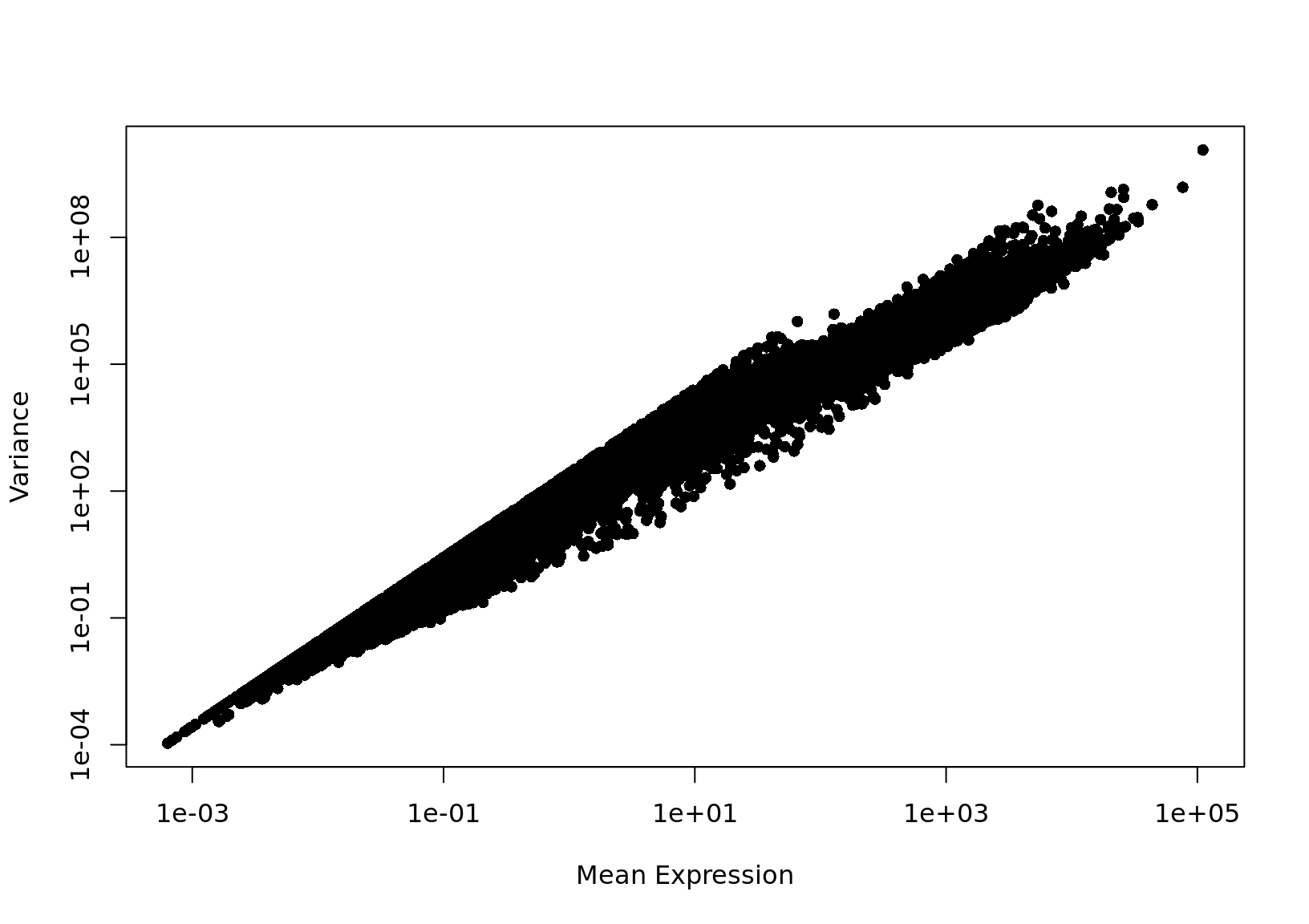
An early method to correct for the relationship between variance and mean expression was proposed by Brennecke et al.. To use the Brennecke method, we first normalize for library size then calculate the mean and the square coefficient of variation (variation divided by the squared mean expression). A quadratic curve is fit to the relationship between these two variables for the ERCC spike-in, and then a chi-square test is used to find genes significantly above the curve. This method is included in the M3Drop package as the Brennecke_getVariableGenes(counts, spikes) function. However, this dataset does not contain spike-ins so we will use the entire dataset to estimate the technical noise.
In the figure below the red curve is the fitted technical noise model and the dashed line is the 95% CI. Pink dots are the genes with significant biological variability after multiple-testing correction.
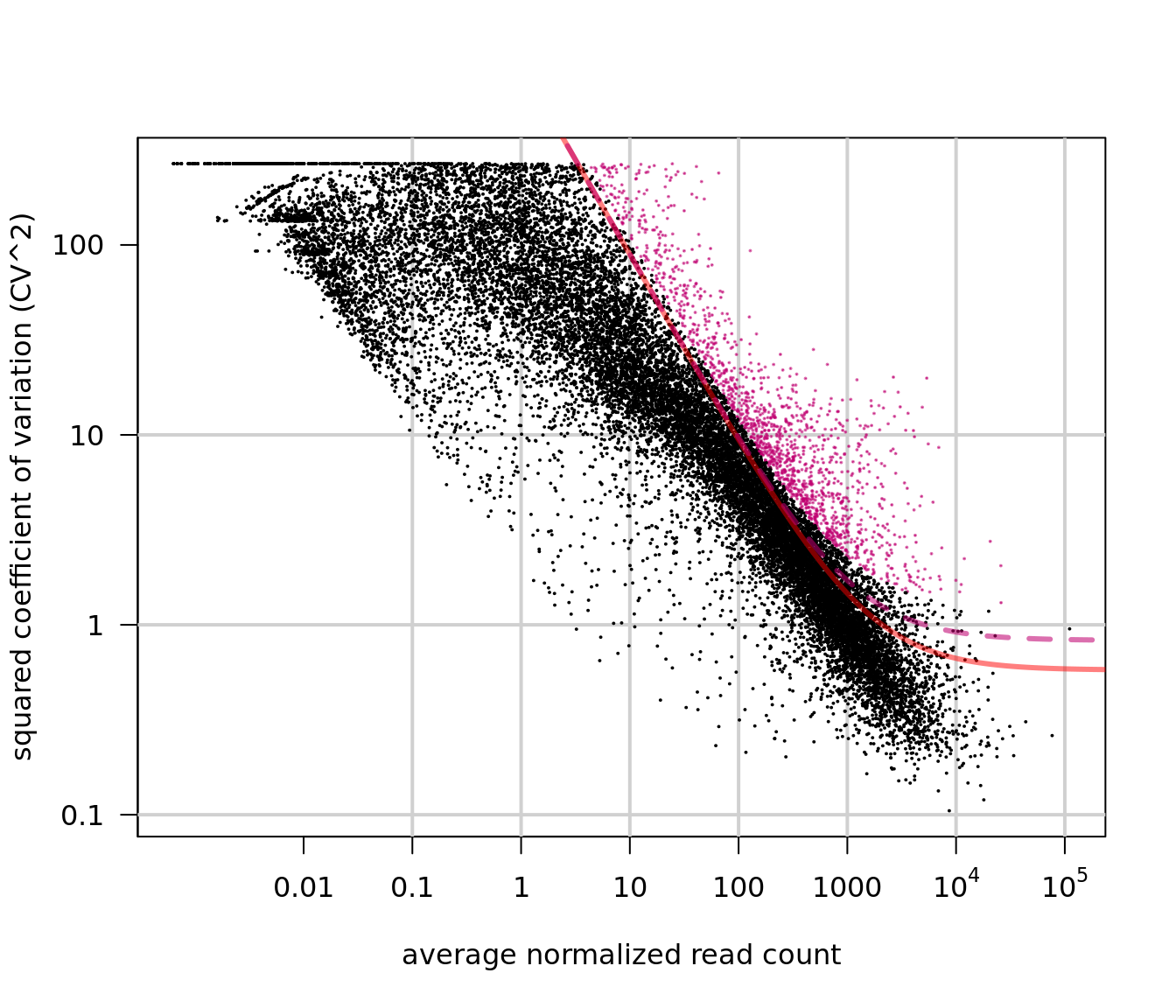
This function returns a matrix of significant genes as well as their estimated effect size (difference between observed and expected coefficient of variation), and their significance as raw p.values and FDR corrected q.values. For now we will just keep the names of the significant HVG genes.
Exercise 3 How many genes were signifcant using BrenneckeGetVariableGenes?
## [1] 13037.8.1.2 Highly Variable Genes - simpleSingleCell method
The Bioconductor
simpleSingleCell
workflow has a great deal of excellent material to help your analyses. Here, we
show how to identify highly variable genes using functionality from the scran
package.
This method assumes that technical variance is captured by a Poisson distribution, and that variance beyond that explained by a Poisson distribution represents biological variance of interest. This approach separates the biological component of the variance from the technical component and thus can rank genes based on their “biological” variance. This model also provides p-values (with FDR adjustment) that can be used to identify the set of “significant” highly variable genes at a given significance level.
### mamke a technical trend of variance based on Poisson
var.fit <- trendVar(deng, parametric=TRUE, loess.args=list(span=0.4), use.spikes = FALSE)
var.out <- decomposeVar(deng, var.fit)
plot(var.out$mean, var.out$total, pch=16, cex=0.6, xlab="Mean log-expression",
     ylab="Variance of log-expression")
points(var.out$mean[isSpike(deng)], var.out$total[isSpike(deng)], col="red", pch=16)
curve(var.fit$trend(x), col="dodgerblue", add=TRUE, lwd=2)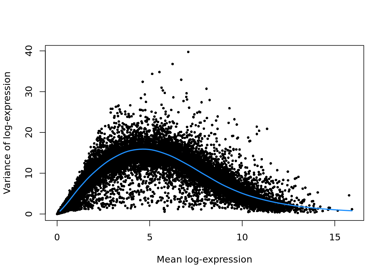
chosen.genes <- order(var.out$bio, decreasing=TRUE)[1:10]
plotExpression(deng, rownames(var.out)[chosen.genes],
               point_alpha=0.5, jitter_type="jitter")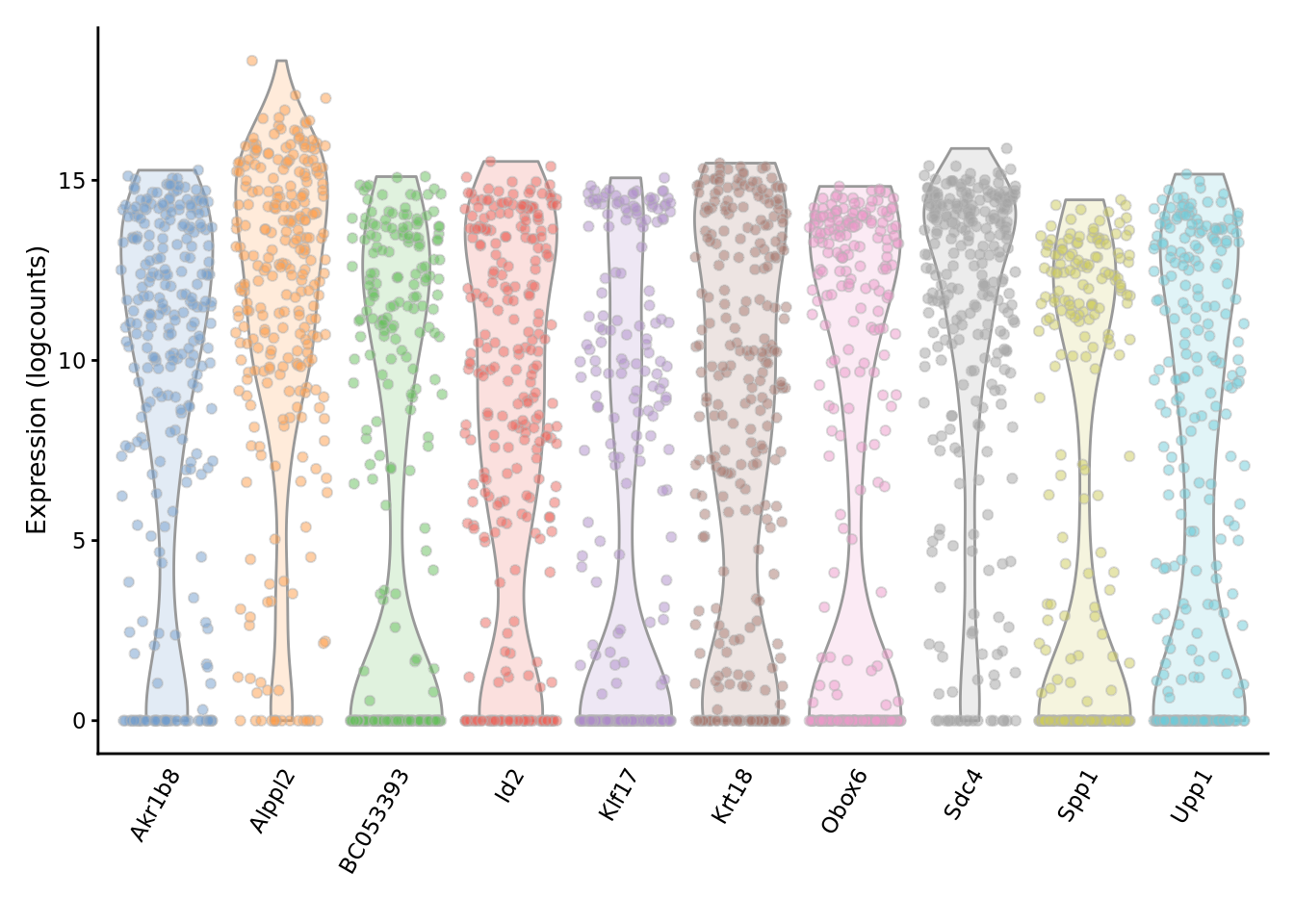
top.dec <- var.out[order(var.out$bio, decreasing=TRUE),]
                                        # the highly variable genes with largest biological components
head(top.dec)
## DataFrame with 6 rows and 6 columns
## mean total bio
## <numeric> <numeric> <numeric>
## Obox6 7.0852220910669 39.7469062194493 27.7222625676479
## BC053393 6.23846872763624 36.7868129334449 22.7409221497424
## Krt18 8.06957111931139 30.7163256353151 21.3338604240051
## Upp1 6.70443458808406 32.9196031154138 19.9537242012223
## Akr1b8 9.31035205790714 25.9351262454146 19.563014227718
## Spp1 5.52672835522051 34.8140952020968 19.5492807120572
## tech p.value FDR
## <numeric> <numeric> <numeric>
## Obox6 12.0246436518013 6.67046481158613e-67 4.98750653962295e-64
## BC053393 14.0458907837025 1.89687518927716e-40 5.90955657926056e-38
## Krt18 9.38246521130992 1.28064383710762e-65 9.26649093876163e-63
## Upp1 12.9658789141915 1.39045180596497e-37 3.89865305745004e-35
## Akr1b8 6.37211201769662 2.70679041028919e-99 5.51963779029062e-96
## Spp1 15.2648144900397 9.4641203490752e-29 1.76908069625088e-26##
## FALSE TRUE
## 21124 1307If we set an FDR threshold of 0.1%, this approach identifies around 1300 highly variable genes.
The output of this variance modelling can be used as input to a denoisePCA()
function to compute “denoised” principal components for clustering and other
downstream analyses (details not shown here; please see the simpleSingleCell
workflow).
7.8.1.3 High Dropout Genes
An alternative to finding HVGs is to identify genes with unexpectedly high numbers of zeros. The frequency of zeros, known as the “dropout rate”, is very closely related to expression level in scRNASeq data. Zeros are the dominant feature of single-cell RNASeq data, typically accounting for over half of the entries in the final expression matrix. These zeros predominantly result from the failure of mRNAs failing to be reversed transcribed (Andrews and Hemberg, 2016). Reverse transcription is an enzyme reaction thus can be modelled using the Michaelis-Menten equation:
\[P_{dropout} = 1 - S/(K + S)\]
where \(S\) is the mRNA concentration in the cell (we will estimate this as average expression) and \(K\) is the Michaelis-Menten constant.
Because the Michaelis-Menten equation is a convex non-linear function, genes which are differentially expression across two or more populations of cells in our dataset will be shifted up/right of the Michaelis-Menten model (see Figure below).
K <- 49
S_sim <- 10^seq(from = -3, to = 4, by = 0.05) # range of expression values
MM <- 1 - S_sim / (K + S_sim)
plot(
    S_sim,
    MM,
    type = "l",
    lwd = 3,
    xlab = "Expression",
    ylab = "Dropout Rate",
    xlim = c(1,1000)
)
S1 <- 10 # Mean expression in population 1
P1 <- 1 - S1 / (K + S1) # Dropouts for cells in condition 1
S2 <- 750 # Mean expression in population 2
P2 <- 1 - S2 / (K + S2) # Dropouts for cells in condition 2
points(
    c(S1, S2),
    c(P1, P2),
    pch = 16,
    col = "grey85",
    cex = 3
)
mix <- 0.5 # proportion of cells in condition 1
points(
    S1 * mix + S2 * (1 - mix),
    P1 * mix + P2 * (1 - mix),
    pch = 16,
    col = "grey35",
    cex = 3
)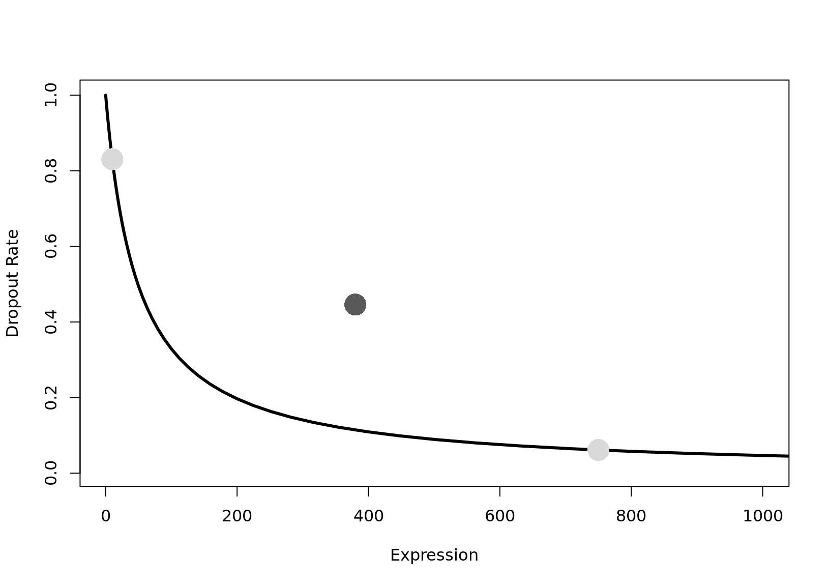
Note: add log="x" to the plot call above to see how this looks on the
log scale, which is used in M3Drop figures.
Exercise 4: Produce the same plot as above with different expression levels (S1 & S2) and/or mixtures (mix).
We use M3Drop to identify significant outliers to the right of the MM curve. We also apply 1% FDR multiple testing correction:
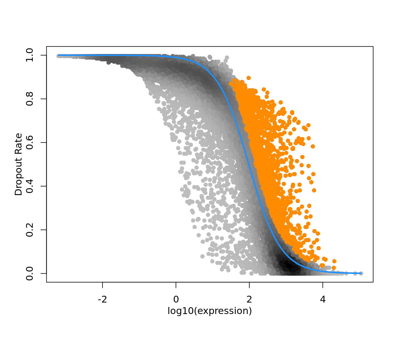
An alternative method is contained in the M3Drop package that is tailored specifically for UMI-tagged data which generally contains many zeros resulting from low sequencing coverage in addition to those resulting from insufficient reverse-transcription. This model is the Depth-Adjusted Negative Binomial (DANB). This method describes each expression observation as a negative binomial model with a mean related to both the mean expression of the respective gene and the sequencing depth of the respective cell, and a variance related to the mean-expression of the gene.
This method is designed to model the raw counts in a dataset directly, and we can extract the appropriate matrix using the “NBumiConvertData” function similar to M3Drop. However, we have an extra step for fitting the model since that is the slowest step of the method and we are currently working on additional methods that can use this model information for other things (such as normalization, co-expression testing, highly variable gene detection).
This method includes a binomial test of the significance of each feature, but since the Deng data is not UMI counts the model does not fit the noise sufficiently and far too many genes will be called as significant. Thus we will take the top 1500 by effect size.
## [1] "Removing 1134 undetected genes."DANB_fit <- NBumiFitModel(deng_int) # DANB is fit to the raw count matrix
# Perform DANB feature selection
DropFS <- NBumiFeatureSelectionCombinedDrop(DANB_fit, method="fdr", qval.thresh=0.01, suppress.plot=FALSE)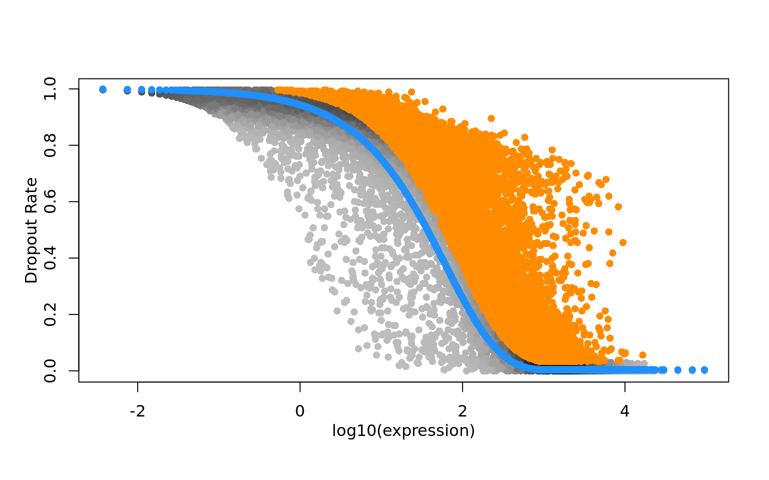
Exercise 5 How many genes were signifcant using NBumiFeatureSelectionCombinedDrop?
## [1] 106947.8.1.4 Residual variance from a (regularized) negative binomial model
In the normalization chapter we introduced the
sctransform approach to using Pearson residuals from an regularized negative
binomial generalized linear model to normalize scRNA-seq data.
The residual variance of genes (i.e. the variance of the Pearson residuals) provides a way to identify highly variable genes, where the “variance” is decoupled from the average level of expression of the gene.
The residual variance is easily accessible from the sctransform output as we
show below.
First, we run sctransform as we did previously.
deng_sparse <- as(counts(deng), "dgCMatrix")
### Genes expressed in at least 5 cells will be kept
sctnorm_data <- sctransform::vst(umi = deng_sparse, min_cells = 1,
                                 cell_attr = as.data.frame(colData(deng)),
latent_var = "log10_total_counts_endogenous")## [1] "y ~ log10_total_counts_endogenous"library(ggplot2)
ggplot(sctnorm_data$gene_attr, aes(residual_variance)) +
geom_histogram(binwidth=0.1) +
geom_vline(xintercept=1, color='red') + xlim(0, 10) +
theme_bw()![]()
sctnorm_data$gene_attr$label <- rownames(sctnorm_data$gene_attr)
ggplot(sctnorm_data$gene_attr, aes(x = gmean, y=residual_variance)) +
  geom_point(alpha = 0.6) +
  geom_point(colour = "firebrick2",
             data = sctnorm_data$gene_attr[sctnorm_data$gene_attr$residual_variance > 3,]) +
  scale_x_log10() +
  geom_hline(yintercept   = 1, size = 3, color = "dodgerblue") +
  geom_label(aes(label = label),
             data = sctnorm_data$gene_attr[sctnorm_data$gene_attr$residual_variance > 30,]) +
theme_bw()![]()
sct_genes <- rownames(sctnorm_data$gene_attr)[sctnorm_data$gene_attr$residual_variance > 4]
table(sctnorm_data$gene_attr$residual_variance > 4)
##
## FALSE TRUE
## 20077 1220If we set a (relatively arbitrary) threshold of a residual variance greater than
three marking a “highly variable gene”, then we identify around 2000 highly
variable genes with this sctransform approach.
[NB: the deng data is extremely high depth for scRNA-seq data, so not the most
applicable dataset for sctransform, but we include this analysis here to
demonstrate the method rather than make any evaluation of its performance in
general.]
Although not explored here, the deviance statistic from the regularized NB GLM fit provides a natural way to select informative features for downstream analyses.
The deviance is a goodness-of-fit statistic for a statistical model. As Wikipedia notes, deviance is a generalization of the idea of using the sum of squares of residuals in ordinary least squares to cases where model-fitting is achieved by maximum likelihood. It plays an important role in exponential dispersion models and generalized linear models, such as the negative binomial model.
However, sctransform does not seem set up to use the model deviance to select
informative features, but we expect this could be a direction the field goes in
the near future. Keep an eye out!
7.8.3 Comparing Methods
We can check whether the identified features really do represent genes differentially expressed between cell-types in this dataset.
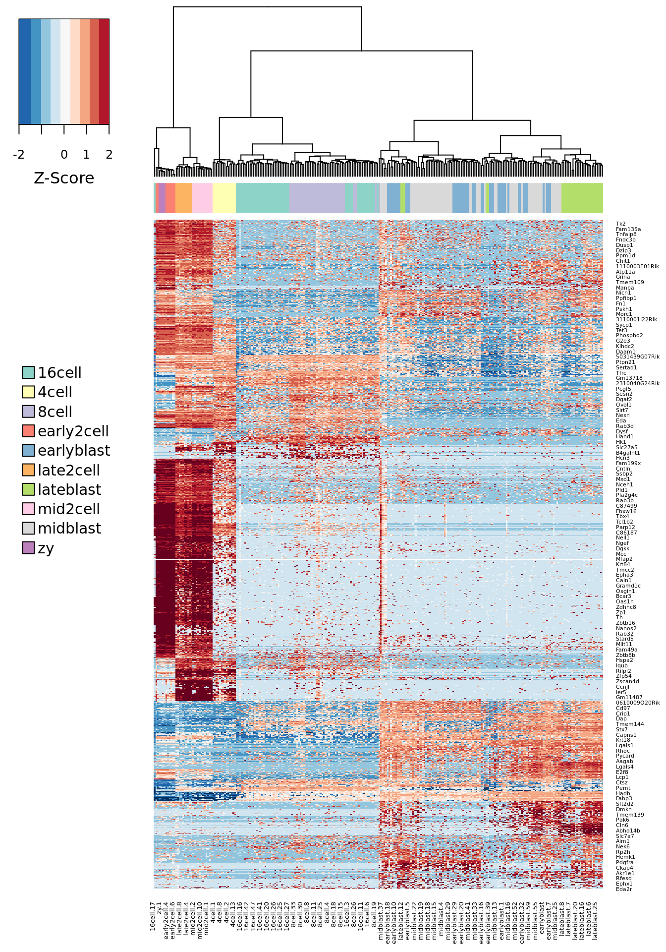
We can also consider how consistent each feature selection method is with the others using the Jaccard Index:
Exercise 6
Plot the expression of the features for each of the other methods. Which appear to be differentially expressed? How consistent are the different methods for this dataset?
Jaccard index comparison of sets of informative features:
list_of_features <- list(
  M3Drop_genes,
  DANB_genes,
  HVG_genes,
  simplesinglecell_genes,
  sct_genes
)
Out <- matrix(
    0,
    ncol = length(list_of_features),
    nrow = length(list_of_features)
)
for(i in 1:length(list_of_features) ) {
    for(j in 1:length(list_of_features) ) {
        Out[i,j] <- sum(list_of_features[[i]] %in% list_of_features[[j]])/
            length(unique(c(list_of_features[[i]], list_of_features[[j]])))
     }
}
colnames(Out) <- rownames(Out) <- c("M3Drop", "DANB", "Brennecke", "simpleSingleCell", "sctransform")
Out
## M3Drop DANB Brennecke simpleSingleCell
## M3Drop 1.0000000 0.38019061 0.4152905 0.14615908
## DANB 0.3801906 1.00000000 0.2283346 0.09868187
## Brennecke 0.4152905 0.22833459 1.0000000 0.15019157
## simpleSingleCell 0.1461591 0.09868187 0.1501916 1.00000000
## sctransform 0.2343257 0.21801471 0.2718985 0.26034913
## sctransform
## M3Drop 0.2343257
## DANB 0.2180147
## Brennecke 0.2718985
## simpleSingleCell 0.2603491
## sctransform 1.00000007.8.4 sessionInfo()
## R version 3.6.0 (2019-04-26)
## Platform: x86_64-pc-linux-gnu (64-bit)
## Running under: Ubuntu 18.04.3 LTS
##
## Matrix products: default
## BLAS:   /usr/lib/x86_64-linux-gnu/blas/libblas.so.3.7.1
## LAPACK: /usr/lib/x86_64-linux-gnu/lapack/liblapack.so.3.7.1
##
## locale:
##  [1] LC_CTYPE=en_AU.UTF-8       LC_NUMERIC=C
##  [3] LC_TIME=en_AU.UTF-8        LC_COLLATE=en_AU.UTF-8
##  [5] LC_MONETARY=en_AU.UTF-8    LC_MESSAGES=en_AU.UTF-8
##  [7] LC_PAPER=en_AU.UTF-8       LC_NAME=C
##  [9] LC_ADDRESS=C               LC_TELEPHONE=C
## [11] LC_MEASUREMENT=en_AU.UTF-8 LC_IDENTIFICATION=C
##
## attached base packages:
## [1] parallel  stats4    stats     graphics  grDevices utils     datasets
## [8] methods   base
##
## other attached packages:
##  [1] scran_1.12.1                scater_1.12.2
##  [3] ggplot2_3.2.1               Polychrome_1.2.3
##  [5] SingleCellExperiment_1.6.0  SummarizedExperiment_1.14.1
##  [7] DelayedArray_0.10.0         BiocParallel_1.18.1
##  [9] Biobase_2.44.0              GenomicRanges_1.36.1
## [11] GenomeInfoDb_1.20.0         IRanges_2.18.3
## [13] S4Vectors_0.22.1            BiocGenerics_0.30.0
## [15] RColorBrewer_1.1-2          M3Drop_1.10.0
## [17] numDeriv_2016.8-1.1         matrixStats_0.55.0
## [19] scRNA.seq.funcs_0.1.0
##
## loaded via a namespace (and not attached):
##   [1] Rtsne_0.15               ggbeeswarm_0.6.0
##   [3] colorspace_1.4-1         dynamicTreeCut_1.63-1
##   [5] htmlTable_1.13.2         XVector_0.24.0
##   [7] base64enc_0.1-3          BiocNeighbors_1.2.0
##   [9] rstudioapi_0.10          listenv_0.7.0
##  [11] codetools_0.2-16         splines_3.6.0
##  [13] knitr_1.25               Formula_1.2-3
##  [15] cluster_2.1.0            sctransform_0.2.0
##  [17] compiler_3.6.0           dqrng_0.2.1
##  [19] backports_1.1.4          assertthat_0.2.1
##  [21] Matrix_1.2-17            lazyeval_0.2.2
##  [23] limma_3.40.6             BiocSingular_1.0.0
##  [25] acepack_1.4.1            htmltools_0.3.6
##  [27] tools_3.6.0              rsvd_1.0.2
##  [29] igraph_1.2.4.1           gtable_0.3.0
##  [31] glue_1.3.1               GenomeInfoDbData_1.2.1
##  [33] reshape2_1.4.3           dplyr_0.8.3
##  [35] Rcpp_1.0.2               bbmle_1.0.20
##  [37] gdata_2.18.0             nlme_3.1-139
##  [39] DelayedMatrixStats_1.6.1 xfun_0.9
##  [41] stringr_1.4.0            globals_0.12.4
##  [43] irlba_2.3.3              gtools_3.8.1
##  [45] hypergeo_1.2-13          statmod_1.4.32
##  [47] future_1.14.0            edgeR_3.26.8
##  [49] zlibbioc_1.30.0          MASS_7.3-51.1
##  [51] scales_1.0.0             yaml_2.2.0
##  [53] gridExtra_2.3            rpart_4.1-15
##  [55] latticeExtra_0.6-28      stringi_1.4.3
##  [57] checkmate_1.9.4          orthopolynom_1.0-5
##  [59] contfrac_1.1-12          caTools_1.17.1.2
##  [61] rlang_0.4.0              pkgconfig_2.0.3
##  [63] moments_0.14             bitops_1.0-6
##  [65] evaluate_0.14            lattice_0.20-38
##  [67] purrr_0.3.2              htmlwidgets_1.3
##  [69] labeling_0.3             cowplot_1.0.0
##  [71] tidyselect_0.2.5         deSolve_1.24
##  [73] plyr_1.8.4               magrittr_1.5
##  [75] bookdown_0.13            R6_2.4.0
##  [77] gplots_3.0.1.1           Hmisc_4.2-0
##  [79] pillar_1.4.2             foreign_0.8-70
##  [81] withr_2.1.2              mgcv_1.8-28
##  [83] survival_2.43-3          scatterplot3d_0.3-41
##  [85] RCurl_1.95-4.12          nnet_7.3-12
##  [87] future.apply_1.3.0       tibble_2.1.3
##  [89] crayon_1.3.4             KernSmooth_2.23-15
##  [91] rmarkdown_1.15           viridis_0.5.1
##  [93] locfit_1.5-9.1           grid_3.6.0
##  [95] data.table_1.12.2        reldist_1.6-6
##  [97] digest_0.6.21            elliptic_1.4-0
##  [99] munsell_0.5.0            beeswarm_0.2.3
## [101] viridisLite_0.3.0        vipor_0.4.5
References
Anders, Simon, and Wolfgang Huber. 2010. “Differential Expression Analysis for Sequence Count Data.” Genome Biol 11 (10). Springer Nature: R106. https://doi.org/10.1186/gb-2010-11-10-r106.
Bullard, James H, Elizabeth Purdom, Kasper D Hansen, and Sandrine Dudoit. 2010. “Evaluation of Statistical Methods for Normalization and Differential Expression in mRNA-Seq Experiments.” BMC Bioinformatics 11 (1). Springer Nature: 94. https://doi.org/10.1186/1471-2105-11-94.
Buttner, Maren, Zhichao Miao, Alexander Wolf, Sarah A Teichmann, and Fabian J Theis. 2017. “Assessment of Batch-Correction Methods for scRNA-seq Data with a New Test Metric.” bioRxiv, October, 200345.
Hafemeister, Christoph, and Rahul Satija. 2019. “Normalization and variance stabilization of single-cell RNA-seq data using regularized negative binomial regression.” bioRxiv. https://doi.org/10.1101/576827.
Haghverdi, Laleh, Aaron T L Lun, Michael D Morgan, and John C Marioni. 2017. “Correcting Batch Effects in Single-Cell RNA Sequencing Data by Matching Mutual Nearest Neighbours.” bioRxiv, July, 165118.
L. Lun, Aaron T., Karsten Bach, and John C. Marioni. 2016. “Pooling Across Cells to Normalize Single-Cell RNA Sequencing Data with Many Zero Counts.” Genome Biol 17 (1). Springer Nature. https://doi.org/10.1186/s13059-016-0947-7.
Ritchie, Matthew E, Belinda Phipson, Di Wu, Yifang Hu, Charity W Law, Wei Shi, and Gordon K Smyth. 2015. “limma powers differential expression analyses for RNA-sequencing and microarray studies.” Nucleic Acids Research 43 (7). Oxford University Press: e47–e47. https://doi.org/10.1093/nar/gkv007.
Robinson, Mark D, and Alicia Oshlack. 2010. “A Scaling Normalization Method for Differential Expression Analysis of RNA-Seq Data.” Genome Biol 11 (3). Springer Nature: R25. https://doi.org/10.1186/gb-2010-11-3-r25.
William Townes, F, Stephanie C Hicks, Martin J Aryee, and Rafael A Irizarry. 2019. “Feature Selection and Dimension Reduction for Single Cell RNA-Seq based on a Multinomial Model.” bioRxiv. https://doi.org/10.1101/574574.