12 Differential Expression (DE) analysis
12.1 Introduction to DE analysis
12.1.1 Bulk RNA-seq
One of the most common types of analyses when working with bulk RNA-seq data is to identify differentially expressed genes. By comparing the genes that change between two or more conditions, e.g. mutant and wild-type or stimulated and unstimulated, it is possible to characterize the molecular mechanisms underlying the change.
Several different methods, e.g. edgeR and DESeq2 and more, have been developed for bulk RNA-seq and become established as parts of robust and widely-used analysis workflows. Moreover, there are also extensive datasets available where the RNA-seq data has been validated using RT-qPCR. These data can be used to benchmark DE finding algorithms and the available evidence suggests that the algorithms are performing well.
12.1.2 Single cell RNA-seq
In contrast to bulk RNA-seq, in scRNA-seq we often do not have a defined set of experimental conditions. Instead, as was shown in a previous chapter (10.2) we can identify the cell groups by using an unsupervised clustering approach. Once the groups have been identified one can find differentially expressed genes either by comparing the differences in variance between the groups (like the Kruskal-Wallis test implemented in SC3), or by comparing gene expression between clusters in a pairwise manner. In the following chapter we will mainly consider tools developed for pairwise comparisons.
These method may also be applied when comparing cells obtained from different groups or conditions. Such analyses can be complicated by differing cell type proportions between samples (i.e. distinct samples cell populations; the unit of replication in the study). In such cases, it is likely beneficial to identify distinct cell types and conduct differential expression testing between conditions within each cell type.
12.1.3 Differences in Distribution
Unlike bulk RNA-seq, we generally have a large number of samples (i.e. cells) for each group we are comparing in single-cell experiments. Thus we may be able to take advantage of the whole distribution of expression values in each group to identify differences between groups rather than only comparing estimates of mean-expression as is standard for bulk RNASeq.
There are two main approaches to comparing distributions. Firstly, we can use
existing statistical models/distributions and fit the same type of model to the
expression in each group then test for differences in the parameters for each
model, or test whether the model fits better if a particular parameter is allowed
to be different according to group. For instance in Chapter
?? we used edgeR to test whether allowing mean
expression to be different in different batches significantly improved the fit
of a negative binomial model of the data.
Alternatively, we can use a non-parametric test which does not assume that expression values follow any particular distribution, e.g. the Kolmogorov-Smirnov test (KS-test). Non-parametric tests generally convert observed expression values to ranks and test whether the distribution of ranks for one group are signficantly different from the distribution of ranks for the other group. However, some non-parametric methods fail in the presence of a large number of tied values, such as the case for dropouts (zeros) in single-cell RNA-seq expression data. Moreover, if the conditions for a parametric test hold, then it will typically be more powerful than a non-parametric test.
12.1.4 Benchmarking of DE methods for scRNA-seq data
So far there has been one high-quality benchmarking study of single-cell differential expression methods (Soneson and Robinson 2018). The figure below summarises the results from that paper (which is well worth reading in full!):
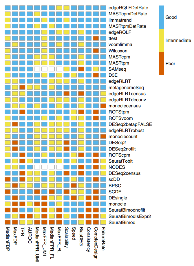
Figure 12.1: Figure 5 reproduced from Soneson and Robinson (2018). Summary of DE method performance across all major evaluation criteria. Criteria and cutoff values for performance categories are available in the Online Methods. Methods are ranked by their average performance across the criteria, with the numerical encoding good = 2, intermediate = 1, poor = 0. NODES and SAMseq do not return nominal P values and were therefore not evaluated in terms of the FPR.
One particularly surprising outcome of this benchmarking study is that almost all methods designed specifically for the analysis of scRNA-seq data are outperformed by established bulk RNA-seq DE methods (edgeR, limma) and standard, classical statistical methods (t-test, Wilcoxon rank-sum tests). MAST (Finak et al. 2015) is the only method designed specifically for scRNA-seq data that performs well in this benchmark. These benchmarking results are a credit to the durability and flexibility of the leading bulk RNA-seq DE methods and a subtle indictment of the land rush of new scRNA-seq methods that were published without adequate comparison to existing bulk RNA-seq methods.
12.1.5 Models of single-cell RNA-seq data
The most common model of RNASeq data is the negative binomial model:
set.seed(1)
hist(
    rnbinom(
        1000,
        mu = 10,
        size = 100),
    col = "grey50",
    xlab = "Read Counts",
    main = "Negative Binomial"
)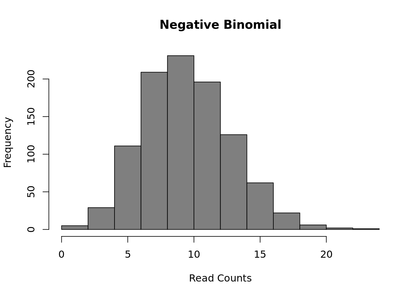
Figure 12.2: Negative Binomial distribution of read counts for a single gene across 1000 cells
Mean: \(\mu = mu\)
Variance: \(\sigma^2 = mu + mu^2/size\)
It is parameterized by the mean expression (mu) and the dispersion (size), which is inversely related to the variance. The negative binomial model fits bulk RNA-seq data very well and it is used for most statistical methods designed for such data. In addition, it has been show to fit the distribution of molecule counts obtained from data tagged by unique molecular identifiers (UMIs) quite well (Grun et al. 2014, Islam et al. 2011).
However, a raw negative binomial model does not necessarily fit full-length transcript data as well due to the high dropout rates relative to the non-zero read counts. For this type of data a variety of zero-inflated negative binomial models have been proposed (e.g. MAST, SCDE).
d <- 0.5;
counts <- rnbinom(
    1000,
    mu = 10,
    size = 100
)
counts[runif(1000) < d] <- 0
hist(
    counts,
    col = "grey50",
    xlab = "Read Counts",
    main = "Zero-inflated NB"
)
Figure 12.3: Zero-inflated Negative Binomial distribution
Mean: \(\mu = mu \cdot (1 - d)\)
Variance: \(\sigma^2 = \mu \cdot (1-d) \cdot (1 + d \cdot \mu + \mu / size)\)
These models introduce a new parameter \(d\), for the dropout rate, to the negative binomial model. As we saw in Chapter 19, the dropout rate of a gene is strongly correlated with the mean expression of the gene. Different zero-inflated negative binomial models use different relationships between mu and d and some may fit \(\mu\) and \(d\) to the expression of each gene independently.
Finally, several methods use a Poisson-Beta distribution which is based on a mechanistic model of transcriptional bursting. There is strong experimental support for this model (Kim and Marioni, 2013) and it provides a good fit to scRNA-seq data but it is less easy to use than the negative-binomial models and much less existing methods upon which to build than the negative binomial model.
a <- 0.1
b <- 0.1
g <- 100
lambdas <- rbeta(1000, a, b)
counts <- sapply(g*lambdas, function(l) {rpois(1, lambda = l)})
hist(
counts,
col = "grey50",
xlab = "Read Counts",
main = "Poisson-Beta"
)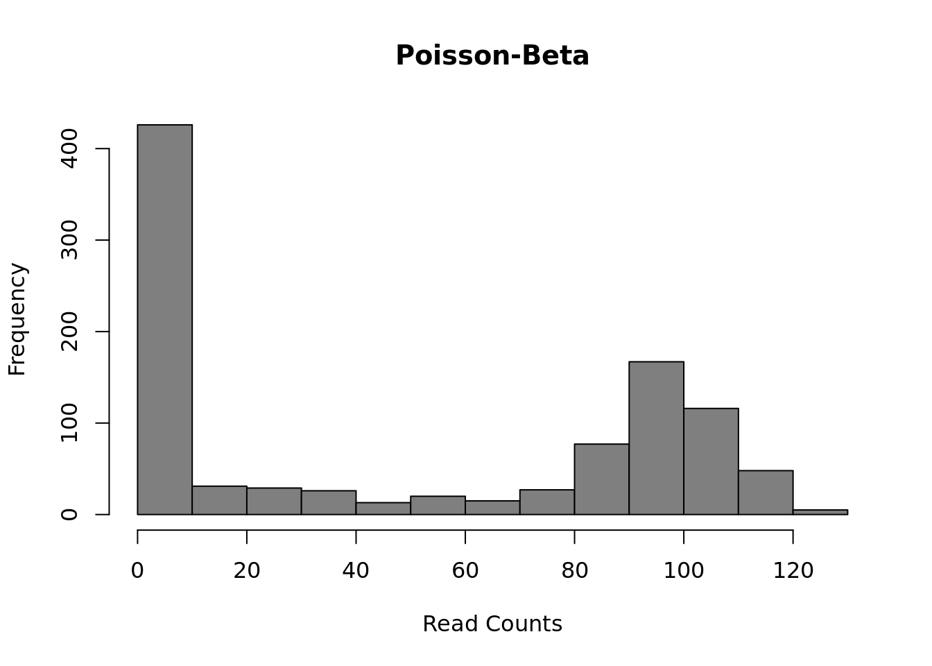 Mean:
\(\mu = g \cdot a / (a + b)\)
Mean:
\(\mu = g \cdot a / (a + b)\)
Variance: \(\sigma^2 = g^2 \cdot a \cdot b/((a + b + 1) \cdot (a + b)^2)\)
This model uses three parameters: \(a\) the rate of activation of transcription; \(b\) the rate of inhibition of transcription; and \(g\) the rate of transcript production while transcription is active at the locus. Differential expression methods may test each of the parameters for differences across groups or only one (often \(g\)).
All of these models may be further expanded to explicitly account for other sources of gene expression differences such as batch-effect or library depth depending on the particular DE algorithm.
Exercise: Vary the parameters of each distribution to explore how they affect the distribution of gene expression. How similar are the Poisson-Beta and Negative Binomial models?
12.2 DE in a real dataset
12.2.1 Introduction
To test different single-cell differential expression methods we will be using the Blischak dataset from Chapters 7-17. For this experiment bulk RNA-seq data for each cell-line was generated in addition to single-cell data. We will use the differentially expressed genes identified using standard methods on the respective bulk data as the ground truth for evaluating the accuracy of each single-cell method. To save time we have pre-computed these for you. You can run the commands below to load these data.
DE <- read.table("data/tung/TPs.txt")
notDE <- read.table("data/tung/TNs.txt")
GroundTruth <- list(
    DE = as.character(unlist(DE)),
    notDE = as.character(unlist(notDE))
)
This ground truth has been produce for the comparison of individual NA19101 to NA19239. Now load the respective single-cell data:
molecules <- read.table("data/tung/molecules.txt", sep = "\t")
anno <- read.table("data/tung/annotation.txt", sep = "\t", header = TRUE)
keep <- anno[,1] == "NA19101" | anno[,1] == "NA19239"
data <- molecules[,keep]
group <- anno[keep,1]
batch <- anno[keep,4]
# remove genes that aren't expressed in at least 6 cells
gkeep <- rowSums(data > 0) > 5;
counts_mat <- as.matrix(data[gkeep,])
# Library size normalization
lib_size <- colSums(counts_mat)
norm <- t(t(counts_mat)/lib_size * median(lib_size))
# Variant of CPM for datasets with library sizes of fewer than 1 mil molecules
Now we will compare various single-cell DE methods. We will focus on methods that performed well in Soneson and Robinson’s (Soneson and Robinson 2018) detailed comparison of differential expression methods for single-cell data. Note that we will only be running methods which are available as R-packages and run relatively quickly.
12.2.2 Kolmogorov-Smirnov test
The types of test that are easiest to work with are non-parametric ones. The most commonly used non-parametric test is the Kolmogorov-Smirnov test (KS-test) and we can use it to compare the distributions for each gene in the two individuals.
The KS-test quantifies the distance between the empirical cummulative distributions of the expression of each gene in each of the two populations. It is sensitive to changes in mean experession and changes in variability. However it assumes data is continuous and may perform poorly when data contains a large number of identical values (eg. zeros). Another issue with the KS-test is that it can be very sensitive for large sample sizes and thus it may end up as significant even though the magnitude of the difference is very small.
)](figures/KS2_Example.png)
Figure 12.4: Illustration of the two-sample Kolmogorov–Smirnov statistic. Red and blue lines each correspond to an empirical distribution function, and the black arrow is the two-sample KS statistic. (taken from here)
Now run the test:
pVals <- apply(
    norm, 1, function(x) {
        ks.test(
            x[group == "NA19101"],
            x[group == "NA19239"]
        )$p.value
    }
)
# multiple testing correction
pVals <- p.adjust(pVals, method = "fdr")
This code “applies” the function to each row (specified by 1) of the expression matrix, data. In the function we are returning just the p.value from the ks.test output. We can now consider how many of the ground truth positive and negative DE genes are detected by the KS-test:
12.2.2.1 Evaluating Accuracy
## [1] 5095## [1] 792## [1] 3190As you can see many more of our ground truth negative genes were identified as DE by the KS-test (false positives) than ground truth positive genes (true positives), however this may be due to the larger number of notDE genes thus we typically normalize these counts as the True positive rate (TPR), TP/(TP + FN), and false discovery rate (FPR), FP/(FP+TP).
tp <- sum(GroundTruth$DE %in% sigDE)
fp <- sum(GroundTruth$notDE %in% sigDE)
tn <- sum(GroundTruth$notDE %in% names(pVals)[pVals >= 0.05])
fn <- sum(GroundTruth$DE %in% names(pVals)[pVals >= 0.05])
tpr <- tp/(tp + fn)
fdr <- fp/(fp + tp)
cat(c(tpr, fdr), "\n")
## 0.7346939 0.801105Now we can see the TPR is OK, but the FDR is very high— much higher than we would normally deem acceptable.
So far we’ve only evaluated the performance at a single significance threshold. Often it is informative to vary the threshold and evaluate performance across a range of values. This is then plotted as a receiver-operating-characteristic curve (ROC) and a general accuracy statistic can be calculated as the area under this curve (AUC). We will use the ROCR package to facilitate this plotting.
# Only consider genes for which we know the ground truth
pVals <- pVals[names(pVals) %in% GroundTruth$DE |
               names(pVals) %in% GroundTruth$notDE]
truth <- rep(1, times = length(pVals));
truth[names(pVals) %in% GroundTruth$DE] = 0;
pred <- ROCR::prediction(pVals, truth)
perf <- ROCR::performance(pred, "tpr", "fpr")
ROCR::plot(perf)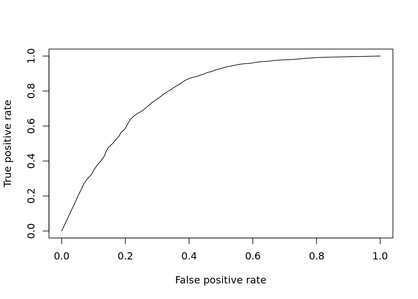
Figure 12.5: ROC curve for KS-test.
## [1] 0.7954796Finally to facilitate the comparisons of other DE methods let’s put this code into a function so we don’t need to repeat it:
DE_Quality_AUC <- function(pVals, plot=TRUE) {
    pVals <- pVals[names(pVals) %in% GroundTruth$DE |
                   names(pVals) %in% GroundTruth$notDE]
    truth <- rep(1, times = length(pVals));
    truth[names(pVals) %in% GroundTruth$DE] = 0;
    pred <- ROCR::prediction(pVals, truth)
    perf <- ROCR::performance(pred, "tpr", "fpr")
    if (plot)
      ROCR::plot(perf)
    aucObj <- ROCR::performance(pred, "auc")
    return(aucObj@y.values[[1]])
}
12.2.3 Wilcoxon/Mann-Whitney-U Test
The Wilcoxon-rank-sum test is another non-parametric test, but tests specifically if values in one group are greater/less than the values in the other group. Thus it is often considered a test for difference in median expression between two groups; whereas the KS-test is sensitive to any change in distribution of expression values.
pVals <- apply(
    norm, 1, function(x) {
        wilcox.test(
            x[group == "NA19101"],
            x[group == "NA19239"]
        )$p.value
    }
)
# multiple testing correction
pVals <- p.adjust(pVals, method = "fdr")
DE_Quality_AUC(pVals)
Figure 12.6: ROC curve for Wilcox test.
## [1] 0.832032612.2.4 edgeR
We’ve already used edgeR for differential expression in Chapter ??. edgeR is based on a negative binomial model of gene expression and uses a generalized linear model (GLM) framework, the enables us to include other factors such as batch to the model.
edgeR, like many DE methods work best with pre-filtering of very lowly
experessed genes. Here, we will keep genes with non-zero expression in at least
30 cells.
The first steps for this analysis then involve
## keep_gene
## FALSE  TRUE
##  4661 11365
dge <- DGEList(
counts = counts_mat[keep_gene,],
norm.factors = rep(1, length(counts_mat[1,])),
group = group
)
group_edgeR <- factor(group)
design <- model.matrix(~ group_edgeR)
dge <- calcNormFactors(dge, method = "TMM")
summary(dge$samples$norm.factors)## Min. 1st Qu. Median Mean 3rd Qu. Max.
## 0.8250 0.9367 0.9584 1.0062 1.0536 1.9618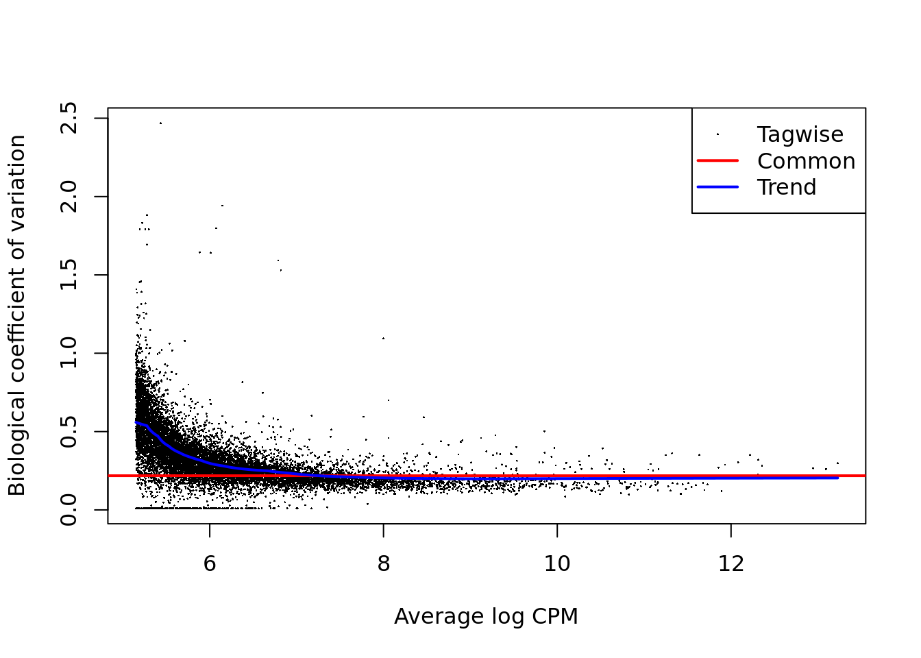
Figure 12.7: Biological coefficient of variation plot for edgeR.
Next we fit a negative binomial quasi-likelihood model for differential expression.
fit <- glmQLFit(dge, design)
res <- glmQLFTest(fit)
pVals <- res$table[,4]
names(pVals) <- rownames(res$table)

pVals <- p.adjust(pVals, method = "fdr")
DE_Quality_AUC(pVals)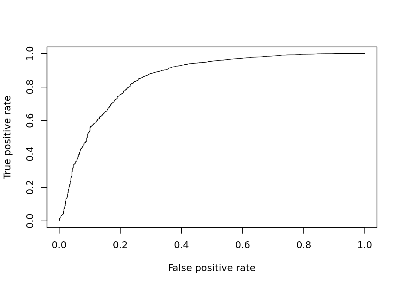
Figure 12.8: ROC curve for edgeR.
## [1] 0.855751412.2.5 MAST
MAST is based on a zero-inflated negative binomial model. It tests for differential expression using a hurdle model to combine tests of discrete (0 vs not zero) and continuous (non-zero values) aspects of gene expression. Again this uses a linear modelling framework to enable complex models to be considered.
log_counts <- log2(counts_mat + 1)
fData <- data.frame(names = rownames(log_counts))
rownames(fData) <- rownames(log_counts);
cData <- data.frame(cond = group)
rownames(cData) <- colnames(log_counts)

obj <- FromMatrix(as.matrix(log_counts), cData, fData)
colData(obj)$cngeneson <- scale(colSums(assay(obj) > 0))
cond <- factor(colData(obj)$cond)

# Model expression as function of condition & number of detected genes
zlmCond <- zlm(~ cond + cngeneson, obj)

summaryCond <- summary(zlmCond, doLRT = "condNA19101")
summaryDt <- summaryCond$datatable

summaryDt <- as.data.frame(summaryDt)
pVals <- unlist(summaryDt[summaryDt$component == "H",4]) # H = hurdle model
names(pVals) <- unlist(summaryDt[summaryDt$component == "H",1])
pVals <- p.adjust(pVals, method = "fdr")
DE_Quality_AUC(pVals)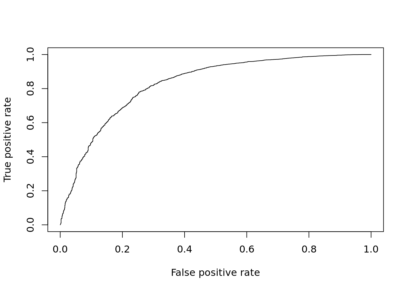
Figure 12.9: ROC curve for MAST.
## [1] 0.828404612.2.6 limma
The limma package implements Empirical Bayes linear models for identifying
differentially expressed genes. Originally developed more microarray data, the
extended limma-voom method has proven to be a very fast and accurate DE method
for bulk RNA-seq data. With its speed and flexibility, limma also performed
well for DE analysis of scRNA-seq data in the benchmarking study mentioned
earlier.
Here we demonstrate how to use limma for DE analysis on these data.
library(limma)
## we can use the same design matrix structure as for edgeR
design <- model.matrix(~ group_edgeR)
colnames(design)
## [1] "(Intercept)" "group_edgeRNA19239"## apply the same filtering of low-abundance genes as for edgeR
keep_gene <- (rowSums(counts_mat > 0) > 29.5 & rowMeans(counts_mat) > 0.2)
summary(keep_gene)## Mode FALSE TRUE
## logical 4661 11365y <- counts_mat[keep_gene, ]
v <- voom(y, design)
fit <- lmFit(v, design)
res <- eBayes(fit)
topTable(res)## logFC AveExpr t P.Value adj.P.Val
## ENSG00000106153 -4.3894938 5.207732 -61.83776 1.048992e-268 1.192180e-264
## ENSG00000022556 -3.6419064 5.368174 -54.24475 1.048481e-238 5.957992e-235
## ENSG00000135549 -2.6370360 4.505792 -37.20177 1.129436e-160 4.278680e-157
## ENSG00000185088 -1.2860563 8.418585 -31.33983 2.410684e-130 6.849355e-127
## ENSG00000170906 0.7971144 8.977602 30.90797 4.732891e-128 1.075786e-124
## ENSG00000184674 -2.1768653 4.129290 -30.73100 4.137245e-127 7.836631e-124
## ENSG00000198825 2.1316479 5.229765 28.20805 1.412125e-113 2.292685e-110
## ENSG00000138035 -1.5188509 6.763545 -27.65932 1.305792e-110 1.855040e-107
## ENSG00000164434 1.8715563 5.782091 24.79885 4.465275e-95 5.638650e-92
## ENSG00000088305 -0.7511259 9.394709 -24.69619 1.615578e-94 1.836104e-91
## B
## ENSG00000106153 599.5015
## ENSG00000022556 531.5858
## ENSG00000135549 354.5934
## ENSG00000185088 287.1727
## ENSG00000170906 281.9116
## ENSG00000184674 278.2672
## ENSG00000198825 247.7511
## ENSG00000138035 241.5441
## ENSG00000164434 205.7273
## ENSG00000088305 204.7427pVals <- res$p.value
names(pVals) <- rownames(y)
pVals <- p.adjust(pVals, method = "fdr")
DE_Quality_AUC(pVals)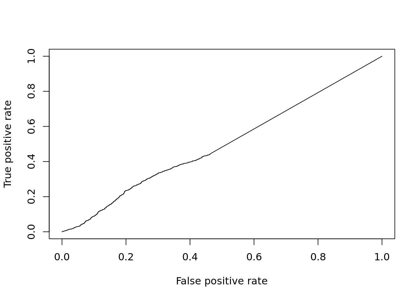
## [1] 0.4984728Q: How does limma compare on this dataset?
12.2.7 Pseudobulk
In this approach, we sum counts across cells from the same condition (here we will use batch within individual) to create “pseudobulk” samples that we will analyse for DE the way we would analyse bulk RNA-seq data. Research continues on benchmarking pseudobulk and single-cell DE approaches, but the suggestion from certain (we think reliable) sources is that pseudobulk approaches are more robust and accurate (and typically very fast) in a range of settings where we’re interested in differences between groups or conditions rather than individual cells.
##                 NA19101.r1 NA19101.r2 NA19101.r3 NA19239.r1 NA19239.r2
## ENSG00000237683         32         23         28         17         33
## ENSG00000187634          1          2          7          5          0
## ENSG00000188976        206        236        204        237        188
## ENSG00000187961         17         32         23         19         19
## ENSG00000187583          2          1          0          1          4
## ENSG00000187642          0          1          0          3          2
##                 NA19239.r3
## ENSG00000237683         15
## ENSG00000187634          7
## ENSG00000188976        391
## ENSG00000187961         25
## ENSG00000187583          1
## ENSG00000187642          2
y <- DGEList(summed)
y <- y[aveLogCPM(y) > 1,]
y <- calcNormFactors(y)
individ <- gsub("\\.r[123]", "", colnames(summed))
design <- model.matrix(~individ)
head(design)## (Intercept) individNA19239
## 1 1 0
## 2 1 0
## 3 1 0
## 4 1 1
## 5 1 1
## 6 1 1## Min. 1st Qu. Median Mean 3rd Qu. Max.
## 0.01609 0.02518 0.03734 0.05450 0.07362 0.14888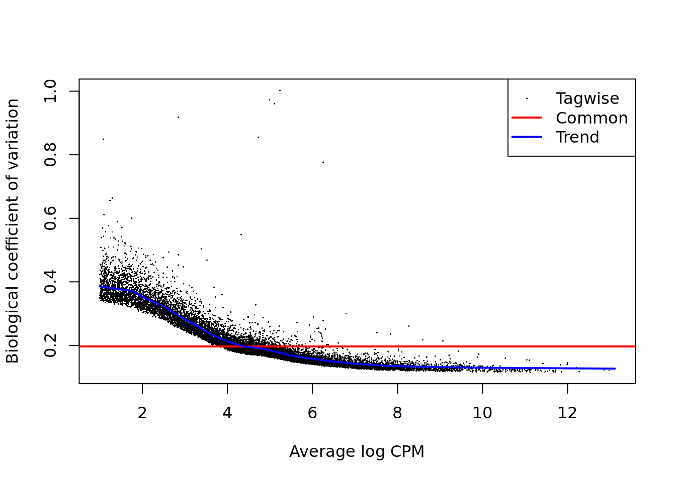
##        individNA19239
## Down              290
## NotSig          11973
## Up                155
pVals <- res$table[,4]
names(pVals) <- rownames(res$table)
pVals <- p.adjust(pVals, method = "fdr")
DE_Quality_AUC(pVals)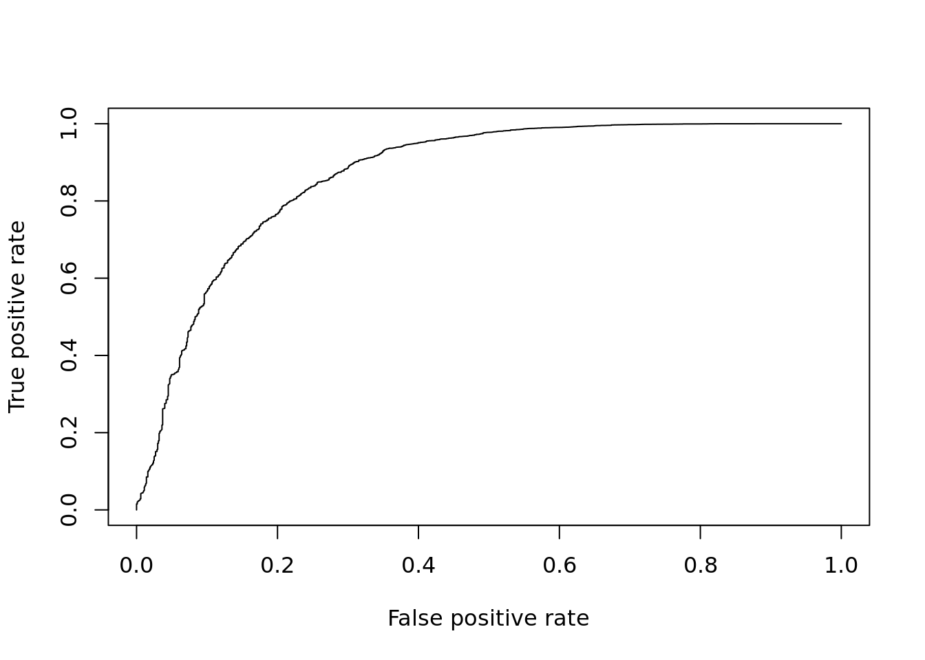
## [1] 0.8685502Q: What do you make of these pseudobulk results? What are the pros and cons of this approach?
12.2.8 Reflection
- What is your overall assessment of the DE methods presented in this chapter?
- When might you choose to use one method in preference to others?
- What caveats or potential problems can you think of with conducting DE testing using approaches like those presented here?
12.2.9 sessionInfo()
## R version 3.6.0 (2019-04-26)
## Platform: x86_64-pc-linux-gnu (64-bit)
## Running under: Ubuntu 18.04.3 LTS
##
## Matrix products: default
## BLAS:   /usr/lib/x86_64-linux-gnu/blas/libblas.so.3.7.1
## LAPACK: /usr/lib/x86_64-linux-gnu/lapack/liblapack.so.3.7.1
##
## locale:
##  [1] LC_CTYPE=en_AU.UTF-8       LC_NUMERIC=C
##  [3] LC_TIME=en_AU.UTF-8        LC_COLLATE=en_AU.UTF-8
##  [5] LC_MONETARY=en_AU.UTF-8    LC_MESSAGES=en_AU.UTF-8
##  [7] LC_PAPER=en_AU.UTF-8       LC_NAME=C
##  [9] LC_ADDRESS=C               LC_TELEPHONE=C
## [11] LC_MEASUREMENT=en_AU.UTF-8 LC_IDENTIFICATION=C
##
## attached base packages:
## [1] parallel  stats4    stats     graphics  grDevices utils     datasets
## [8] methods   base
##
## other attached packages:
##  [1] ROCR_1.0-7                  gplots_3.0.1.1
##  [3] MAST_1.10.0                 SingleCellExperiment_1.6.0
##  [5] SummarizedExperiment_1.14.1 DelayedArray_0.10.0
##  [7] BiocParallel_1.18.1         matrixStats_0.55.0
##  [9] Biobase_2.44.0              GenomicRanges_1.36.1
## [11] GenomeInfoDb_1.20.0         IRanges_2.18.3
## [13] S4Vectors_0.22.1            BiocGenerics_0.30.0
## [15] edgeR_3.26.8                limma_3.40.6
## [17] scRNA.seq.funcs_0.1.0
##
## loaded via a namespace (and not attached):
##  [1] nlme_3.1-139             bitops_1.0-6
##  [3] progress_1.2.2           tools_3.6.0
##  [5] backports_1.1.4          R6_2.4.0
##  [7] irlba_2.3.3              vipor_0.4.5
##  [9] KernSmooth_2.23-15       hypergeo_1.2-13
## [11] lazyeval_0.2.2           colorspace_1.4-1
## [13] gridExtra_2.3            tidyselect_0.2.5
## [15] prettyunits_1.0.2        moments_0.14
## [17] compiler_3.6.0           orthopolynom_1.0-5
## [19] BiocNeighbors_1.2.0      bookdown_0.13
## [21] caTools_1.17.1.2         scales_1.0.0
## [23] blme_1.0-4               stringr_1.4.0
## [25] digest_0.6.21            minqa_1.2.4
## [27] rmarkdown_1.15           XVector_0.24.0
## [29] scater_1.12.2            pkgconfig_2.0.3
## [31] htmltools_0.3.6          lme4_1.1-21
## [33] highr_0.8                rlang_0.4.0
## [35] DelayedMatrixStats_1.6.1 gtools_3.8.1
## [37] dplyr_0.8.3              RCurl_1.95-4.12
## [39] magrittr_1.5             BiocSingular_1.0.0
## [41] GenomeInfoDbData_1.2.1   Matrix_1.2-17
## [43] Rcpp_1.0.2               ggbeeswarm_0.6.0
## [45] munsell_0.5.0            viridis_0.5.1
## [47] abind_1.4-5              stringi_1.4.3
## [49] yaml_2.2.0               MASS_7.3-51.1
## [51] zlibbioc_1.30.0          Rtsne_0.15
## [53] plyr_1.8.4               grid_3.6.0
## [55] gdata_2.18.0             crayon_1.3.4
## [57] contfrac_1.1-12          lattice_0.20-38
## [59] splines_3.6.0            hms_0.5.1
## [61] locfit_1.5-9.1           zeallot_0.1.0
## [63] knitr_1.25               pillar_1.4.2
## [65] boot_1.3-20              reshape2_1.4.3
## [67] glue_1.3.1               evaluate_0.14
## [69] data.table_1.12.2        deSolve_1.24
## [71] vctrs_0.2.0              nloptr_1.2.1
## [73] gtable_0.3.0             purrr_0.3.2
## [75] assertthat_0.2.1         ggplot2_3.2.1
## [77] xfun_0.9                 rsvd_1.0.2
## [79] viridisLite_0.3.0        tibble_2.1.3
## [81] elliptic_1.4-0           beeswarm_0.2.3
## [83] statmod_1.4.32
References
Finak, Greg, Andrew McDavid, Masanao Yajima, Jingyuan Deng, Vivian Gersuk, Alex K Shalek, Chloe K Slichter, et al. 2015. “MAST: a flexible statistical framework for assessing transcriptional changes and characterizing heterogeneity in single-cell RNA sequencing data.” Genome Biology 16 (1): 1–13. https://doi.org/10.1186/s13059-015-0844-5.
Soneson, Charlotte, and Mark D Robinson. 2018. “Bias, robustness and scalability in single-cell differential expression analysis.” Nature Methods, February. Nature Publishing Group, a division of Macmillan Publishers Limited. All Rights Reserved. https://doi.org/10.1038/nmeth.4612.