5 Processing raw scRNA-seq data
5.1 Generating fastq files from BCLs
BCLs (Illumina sequencer’s base call files) are binary files with raw sequencing
data generated from sequencers. If your data processing starts BCLs you will
need to make fastq files from the BCL files. More on BCL
format.
For others, you may have received the fastq files from your sequencing
facilities or collaborators, you can refer to Section 5.2 for pre-processing
on fastq files.
5.1.1 Demultiplexing
In cases where multiple sample libraries are pooled together for sequencing on one lane of a flowcell to reduce seqeuncing cost, we demultiplex the samples by their sample index in the step of making fastq files from BCLs. Sample indices are ‘barcodes’ for multiplexed samples which have been constructed in the read structure during the library preparation.
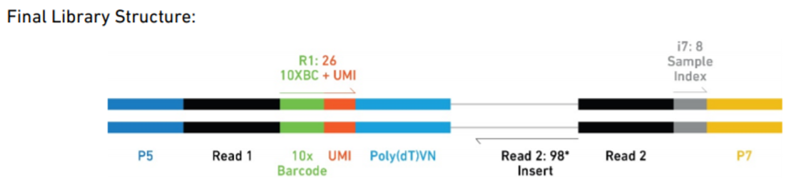
Figure 2.3: Example 10X Final Library Structure
5.1.2 cellranger mkfastq
If you are working with 10X Genomiec data, it is best to use the cellranger mkfastq pipleline, which wraps Illumina’s bcl2fastq and provides a number of
convenient features designed specifically for 10X data format. In order to
demultiplex samples, you would also need the sample_sheet.csv file which tells
the mkfastq pipeline which libraries are sequenced on which lanes of the
flowcell and what sample index sets they have. For example when you have
multiple libraries sequenced on one lane here: 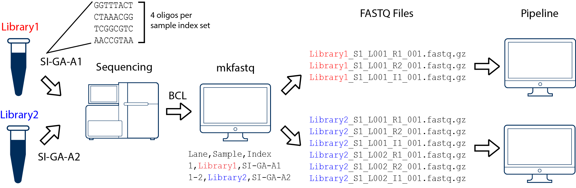
With cellranger mkfastq, you can provide a simpleSampleSheet.csv file that has:
Lane    Sample    Index
1    test_sample    SI-P03-C9
1    test_sample2   SI-P03-A3
...
SI-P03-C9 and SI-P03-A3 are the 10x sample index set names. Each of them
corresponds to a mix of 4 unique oligonucleotides so that the i7 index read is
balanced across all 4 bases during sequencing. There are a list of 96 sample
index sets and you can use any ones of them to ‘tag’ your samples.
An example command to run cellranger mkfastq
/mnt/Software/cellranger/cellranger-3.0.2/cellranger mkfastq \
        --run ./input.runs.folder/ --samplesheet {input.samplesheet.csv} \
        --id run_id \
        --qc --project MAXL_2019_LIM_organoid_RNAseq \
        --output-dir data/fastq_path/ \
        --jobmode=local --localcores=20 --localmem=50 1> {log}
After mkfastq, you end up with each sample’s fastq files from each sequencing lanes:
test_sample_S1_L001_I1_001.fastq.gz
test_sample_S1_L001_R1_001.fastq.gz
test_sample_S1_L001_R2_001.fastq.gz
test_sample2_S2_L001_I1_001.fastq.gz
test_sample2_S2_L001_R1_001.fastq.gz
test_sample2_S2_L001_R2_001.fastq.gz
5.1.3 Illumina bcl2fastq
You can also use Illumina’s bcl2fastq tool directly and it is more generally
applicable. bcf2fastq converts BCLs to fastqs while optionally demultiplexing
sequencing data. Find the documentation of the tool
here;
training videos
may also help to come to grips with using this tool.

Figure 2.4: Sample Demultiplexing
SampleSheet.csv file like this:
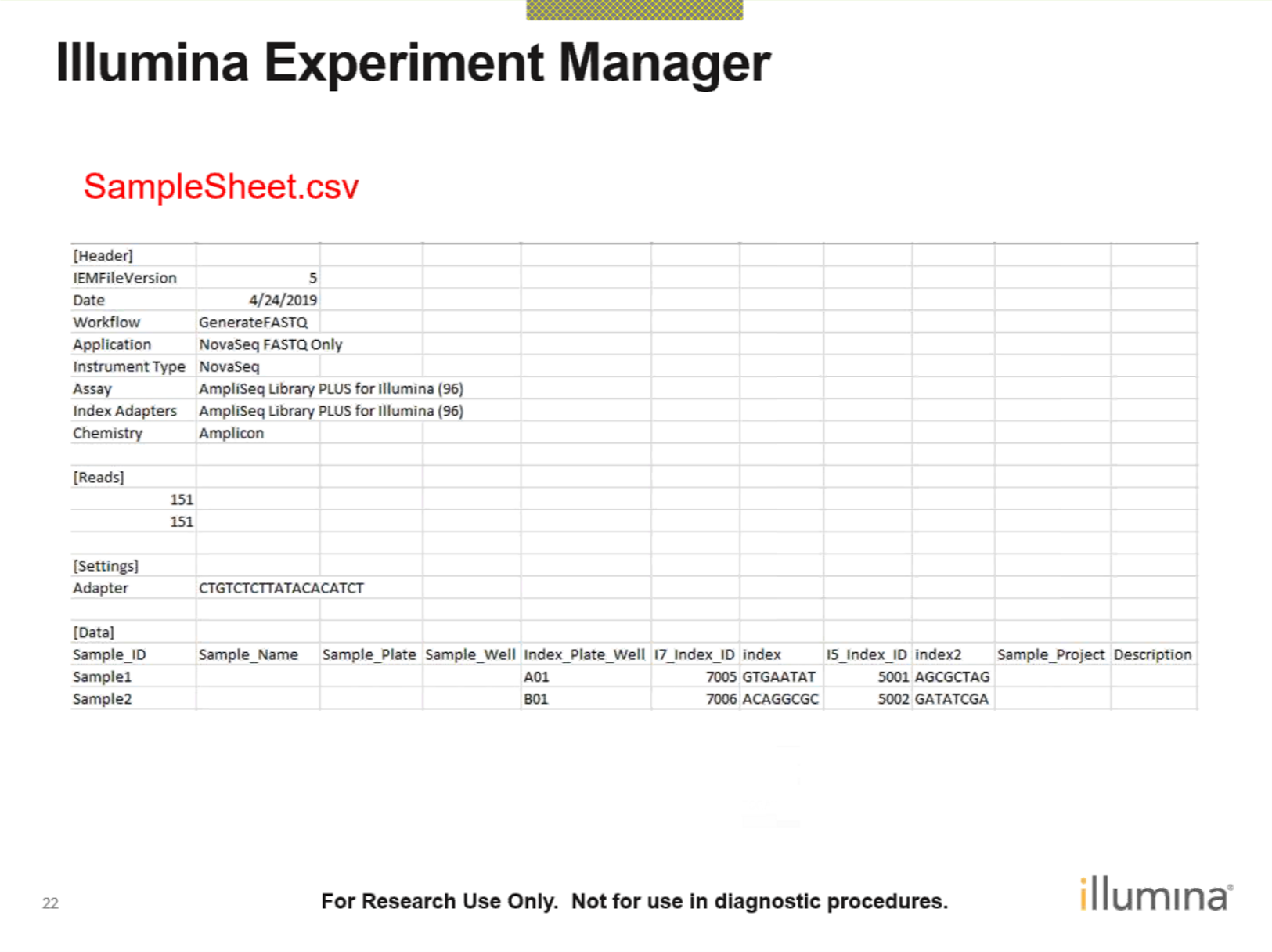
Figure 2.5: SampleSheet.csv file
This information should come from your sequencing facilities. Running
bcl2fastq can then be done like this:
/usr/local/bin/bcl2fastq --runfolder-dir <RunFolder>
--output-dir <BaseCalls>
The output fastq files are names as
SampleName_SampleNumber_Lane_Read_001.fastq.gz same with cellranger mkfastq
output. (eg: Sample1_S1_L001_R1_001.fastq.gz)
5.2 FastQC
Once you’ve obtained your single-cell RNA-seq data, the first thing you need to do with it is check the quality of the reads you have sequenced. For this task, today we will be using a tool called FastQC. FastQC is a quality control tool for sequencing data, which can be used for both bulk and single-cell RNA-seq data. FastQC takes sequencing data as input and returns a report on read quality. Copy and paste this link into your browser to visit the FastQC website:
https://www.bioinformatics.babraham.ac.uk/projects/fastqc/
This website contains links to download and install FastQC and documentation on the reports produced. Scroll down the webpage to ‘Example Reports’ and click ‘Good Illumina Data’. This gives an example of what an ideal report should look like for high quality Illumina reads data.
Now let’s make a FastQC report ourselves.
Today we will be performing our analysis using a single cell from an mESC dataset produced by (Kolodziejczyk et al. 2015). The cells were sequenced using the SMART-seq2 library preparation protocol and the reads are paired end.
Note You will have to download the files (both ERR522959_1.fastq and ERR522959_2.fastq) and create Share directory yourself to run the commands. You can find the files here: https://www.ebi.ac.uk/arrayexpress/experiments/E-MTAB-2600/samples/
Now let’s look at the files:
Task 1: Try to work out what command you should use to produce the FastQC report. Hint: Try executing
This command will tell you what options are available to pass to FastQC. Feel free to ask for help if you get stuck! If you are successful, you should generate a .zip and a .html file for both the forwards and the reverse reads files. Once you have been successful, feel free to have a go at the next section.
5.2.1 Solution and Downloading the Report
If you haven’t done so already, generate the FastQC report using the commands below:
Once the command has finished executing, you should have a total of four files - one zip file for each of the paired end reads, and one html file for each of the paired end reads. The report is in the html file. To view it, we will need to get it onto your computer using either filezilla or scp. Ask an instructor if you are having difficulties.
Once the file is on you computer, click on it. Your FastQC report should open. Have a look through the file. Remember to look at both the forwards and the reverse end read reports! How good quality are the reads? Is there anything we should be concerned about? How might we address those concerns?
5.2.2 10X fastq qualities checks
If you have generated the fastq files from cellranger mkfastq as we discussed before, you can get a list of quality metrics from the output files. First thing to look at will be qc_summary.json file which contains lines like this:
"sample_qc": {
  "Sample1": {
    "5": {
      "barcode_exact_match_ratio": 0.9336158258904611,
      "barcode_q30_base_ratio": 0.9611993091728814,
      "bc_on_whitelist": 0.9447542078230667,
      "mean_barcode_qscore": 37.770630795934,
      "number_reads": 2748155,
      "read1_q30_base_ratio": 0.8947676653366835,
      "read2_q30_base_ratio": 0.7771883245304577
    },
    "all": {
      "barcode_exact_match_ratio": 0.9336158258904611,
      "barcode_q30_base_ratio": 0.9611993091728814,
      "bc_on_whitelist": 0.9447542078230667,
      "mean_barcode_qscore": 37.770630795934,
      "number_reads": 2748155,
      "read1_q30_base_ratio": 0.8947676653366835,
      "read2_q30_base_ratio": 0.7771883245304577
    }
  }
}
5.3 Trimming Reads
Fortunately there is software available for read trimming. Today we will be using Trim Galore!. Trim Galore! is a wrapper for the reads trimming software cutadapt and fastqc.
Read trimming software can be used to trim sequencing adapters and/or low quality reads from the ends of reads. Given we noticed there was some adaptor contamination in our FastQC report, it is a good idea to trim adaptors from our data.
Task 2: What type of adapters were used in our data? Hint: Look at the FastQC report ‘Adapter Content’ plot.
Now let’s try to use Trim Galore! to remove those problematic adapters. It’s a good idea to check read quality again after trimming, so after you have trimmed your reads you should use FastQC to produce another report.
Task 3: Work out the command you should use to trim the adapters from our data.
Hint 1: You can use the following command to find out what options you can pass to Trim Galore.
_Hint 2:** Read through the output of the above command carefully. The adaptor used in this experiment is quite common. Do you need to know the actual sequence of the adaptor to remove it?
Task 3: Produce a FastQC report for your trimmed reads files. Is the adapter contamination gone?
Once you think you have successfully trimmed your reads and have confirmed this by checking the FastQC report, feel free to check your results using the next section.
5.3.1 Solution
You can use the command(s) below to trim the Nextera sequencing adapters:
mkdir fastqc_trimmed_results
trim_galore --nextera -o fastqc_trimmed_results Share/ERR522959_1.fastq Share/ERR522959_2.fastq
Remember to generate new FastQC reports for your trimmed reads files! FastQC should now show that your reads pass the ‘Adaptor Content’ plot. Feel free to ask one of the instructors if you have any questions.
Congratulations! You have now generated reads quality reports and performed adaptor trimming. In the next lab, we will use STAR and Kallisto to align our trimmed and quality-checked reads to a reference transcriptome.
5.4 Fastp
Fastp is an ‘all-in-one’ pre-processing
tool to run on fastq files which has integrated a lot aspects of quality
profiling for both before and after filtering data (quality curves, base
contents, KMER, Q20/Q30, GC Ratio, duplication, adapter contents and etc.
Example usage:
mkdir fastp_results

fastp -i Share/ERR522959_1.fastq  -I Share/ERR522959_2.fastq \
      -o fastp_results/ERR522959_1.fastp.fastq -O fastp_results/ERR522959_1.fastp.fastq \
      --length_required 20 --average_qual 20 --detect_adapter_for_pe --correction \
      -h fastp_results/ERR522959.html -j fastp_results/ERR522959.json
5.5 Read alignment and gene expression quantification
Now we have trimmed our reads and established that they are of good quality, we would like to map them to a reference genome. This process is known as alignment. Some form of alignment is generally required if we want to quantify gene expression or find genes which are differentially expressed between samples.
Many tools have been developed for read alignment. STAR (Dobin et al. 2013) is one of most popularly used tools in RNA-seq read alignment. There are a bunch of alignment and gene expression quantification tools that are designed specifically for single-cell RNA-seq data too. Depending on your single-cell RNA-seq protocols used and the datasets generated, you can go with the following two workflows presented here for full-length or tag-based datasets.
Thus, today we will focus on two alignment tools: STAR and Kallisto-BUStools, and we will discuss other available tools at the end of this chapter.
5.6 Full-length transcript datasets
If your single-cell RNA-seq dataset is from plate-based protocol like Smart-seq2, then your dataset can be aligned and quantifified just like a bulk RNA-seq datasest. Each cell has a proper pair (if it’s paired-end sequncing) of fastq files (there are no CB/UMI tags in the reads). STAR is a good choice for alignment (other good choices could be Subread or Hisat2).
5.6.1 Using STAR to align reads
STAR tries to find the longest possible sequence which matches one or more sequences in the reference genome. For example, in the figure below, we have a read (blue) which spans two exons and an alternative splicing junction (purple). STAR finds that the first part of the read is the same as the sequence of the first exon, whilst the second part of the read matches the sequence in the second exon. Because STAR is able to recognise splicing events in this way, it is described as a ‘splice aware’ aligner.
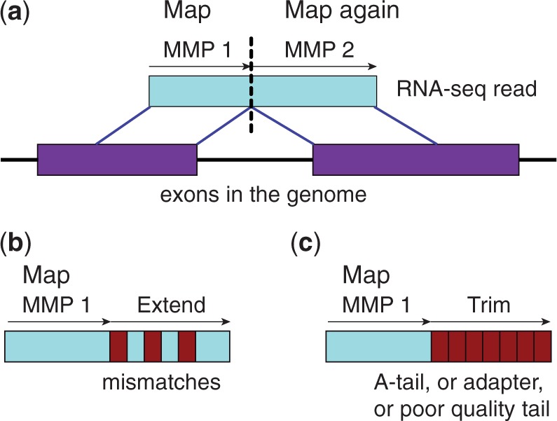
Figure 2.3: Diagram of how STAR performs alignments, taken from Dobin et al.
Usually STAR aligns reads to a reference genome, potentially allowing it to detect novel splicing events or chromosomal rearrangements.
5.6.2 Expression quantification
Now you have your aligned reads in a .bam file for your single cells. The next
step is to quantify the expression level of each gene per cell. We can use one
of the tools which has been developed for bulk RNA-seq data, e.g.
HT-seq or
FeatureCounts which do ‘simple’
counting of reads overlapping with genomic features.
Here we demostrate an example with featureCounts, that counts mapped reads for
genomic features such as genes, exons, promoter, gene bodies, genomic bins and
chromosomal locations.
# include multimapping
<featureCounts_path>/featureCounts -O -M -Q 30 -p -a hg_annotations.gtf -o outputfile ERR522959.bam

# exclude multimapping
<featureCounts_path>/featureCounts -Q 30 -p -a hg_annotations.gtf -o outputfile ERR522959.bam
Then you will have your read counts gene expression matrix that’s ready for downstream analysis.
5.7 Tag-based datasets
If your dataset is tag-based, for example 10X dataset, then you typically have sequences in R1 that entirely encode for read identities such as Cell Barcode and UMI tags. In most cases, all your cell reads (for 1k-10K cells) are in one set of fastq files. Instead of trying to demultiplex all cells into separate fastqs then do alignment and quantification, we can use tools that take care of this for you. In the following steps, we use Kallisto with bustools for generating the gene expression quantification matrix for your tag-based datasets.
5.7.1 Cellranger count
If you work with 10X dataset, cellranger count pipeline may just work well for
you. It comes with cellranger software suite with convenient features for 10X
datasets. It takes the fastqs of a sample, and uses STAR to align all cells’
reads. It also includes reads filtering, barcode counting, and UMI counting. The
output of this pipeline includes the aligned.bam file and the quantified gene
expression matrix in both filtered and raw format. In V3, it has adopted the
EmptyDroplet method (Lun et al., 2018), an algorithm that tries distinguish
true cell barcodes from barcodes associated with droplets that did not contain a
cell (i.e. empty droplets). (More details in Section 5.9 ). The filtered gene
expression matrix by cellranger count V3 only includes the true cell barcodes
determined by EmptyDroplet method.
5.7.2 Kallisto/bustools and pseudo-alignment
STAR is a reads aligner, whereas Kallisto is a pseudo-aligner (Bray et al. 2016). The main difference between aligners and pseudo-aligners is that whereas aligners map reads to a reference, pseudo-aligners map k-mers to a reference.
5.7.3 What is a k-mer?
A k-mer is a sequence of length k derived from a read. For example, imagine we have a read with the sequence ATCCCGGGTTAT and we want to make 7-mers from it. To do this, we would find the first 7-mer by counting the first seven bases of the read. We would find the second 7-mer by moving one base along, then counting the next seven bases. Below shows all the 7-mers that could be derived from our read:
ATCCCGGGTTAT

ATCCCGG
 TCCCGGG
  CCCGGGT
   CCGGGTT
    CGGGTTA
     GGGTTAT
5.7.4 Why map k-mers rather than reads?
There are two main reasons:
Pseudo-aligners use k-mers and a computational trick to make pseudo-alignment much faster than traditional aligners. If you are interested in how this is acheived, see (Bray et al. 2016) for details.
Under some circumstances, pseudo-aligners may be able to cope better with sequencing errors than traditional aligners. For example, imagine there was a sequencing error in the first base of the read above and the A was actually a T. This would impact on the pseudo-aligners ability to map the first 7-mer but none of the following 7-mers.
5.7.5 Kallisto’s pseudo mode
Kallisto has a specially designed mode for pseudo-aligning reads from single-cell RNA-seq experiments. Unlike STAR, Kallisto psuedo-aligns to a reference transcriptome rather than a reference genome. This means Kallisto maps reads to splice isoforms rather than genes. Mapping reads to isoforms rather than genes is especially challenging for single-cell RNA-seq for the following reasons:
- Single-cell RNA-seq is lower coverage than bulk RNA-seq, meaning the total amount of information available from reads is reduced.
- Many single-cell RNA-seq protocols have 3’ coverage bias, meaning if two isoforms differ only at their 5’ end, it might not be possible to work out which isoform the read came from.
- Some single-cell RNA-seq protocols have short read lengths, which can also mean it is not possible to work out which isoform the read came from.
Kallisto’s pseudo mode takes a slightly different approach to pseudo-alignment. Instead of aligning to isoforms, Kallisto aligns to equivalence classes. Essentially, this means if a read maps to multiple isoforms, Kallisto records the read as mapping to an equivalence class containing all the isoforms it maps to. Figure 2 shows a diagram which helps explain this.
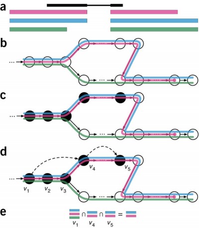
Figure 2.4: Overview of kallisto, The input consists of a reference transcriptome and reads from an RNA-seq experiment. (a) An example of a read (in black) and three overlapping transcripts with exonic regions as shown. (b) An index is constructed by creating the transcriptome de Bruijn Graph (T-DBG) where nodes (v1, v2, v3, … ) are k-mers, each transcript corresponds to a colored path as shown and the path cover of the transcriptome induces a k-compatibility class for each k-mer. (c) Conceptually, the k-mers of a read are hashed (black nodes) to find the k-compatibility class of a read. (d) Skipping (black dashed lines) uses the information stored in the T-DBG to skip k-mers that are redundant because they have the same k-compatibility class. (e) The k-compatibility class of the read is determined by taking the intersection of the k-compatibility classes of its constituent k-mers. Taken from Bray et al (2016).
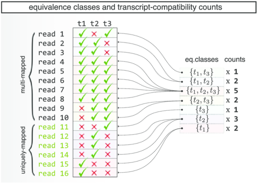
Figure 2.5: A diagram explaining Kallisto’s Equivalence Classes, taken from Ntranos et al.
Note Instead of using gene or isoform expression estimates in downstream analysis such as clustering, equivalence class counts can be used instead, in this course, we focus on using gene level estimation.
5.7.6 Running kallisto pseudo-alignment and BUStools
Today, we will talk about doing single-cell pseudo-alignemnt and gene level
quantification with Kallisto|BUStools. See
https://pachterlab.github.io/kallisto/manual for details.
As for STAR, you will need to produce an index for Kallisto before the pseudo-alignment step.
Use the below command to produce the Kallisto index. Use the Kallisto manual (https://pachterlab.github.io/kallisto/manual) to work out what the options do in this command.
mkdir indices/Kallisto
kallisto index -i indices/Kallisto/GRCm38.idx Share/mouse/Ensembl.GRCm38.96/Mus_musculus.GRCm38.cdna.all.fa.gz
In this step, an index is constructed by creating the transcriptome de Bruijn Graph (T-DBG).
5.7.6.1 BUS format
BUS is a binary file format designed for UMI-tagged single-cell datasets with
pseudo-aligned reads labelled with CB and UMI tags.
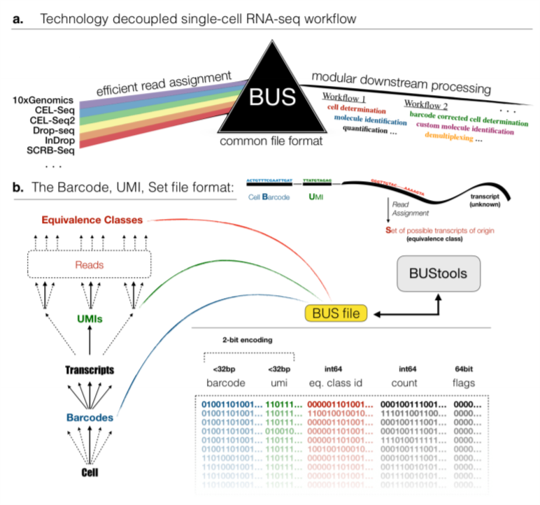
Figure 2.7: BUS format, taken from Melsted,Páll et al.
We do kallisto bus on the fastqs of single cells to generate the BUS file and
then use BUStools on the generated bus files to get a gene level
quantification.
Check the list of technologies supported by Kallisto BUStools by kallisto bus -l Use the below command to perform pseudo-alignment and generate bus files for
single-cell sequencing data. -x argument specifies the technology.
List of supported single-cell technologies

short name       description
----------       -----------
10xv1            10x version 1 chemistry
10xv2            10x version 2 chemistry
10xv3            10x version 3 chemistry
CELSeq           CEL-Seq
CELSeq2          CEL-Seq version 2
DropSeq          DropSeq
inDrops          inDrops
SCRBSeq          SCRB-Seq
SureCell         SureCell for ddSEQ
mkdir results/Kallisto
kallisto bus -i indices/Kallisto/GRCm38.idx -o results/Kallisto/output_bus -x '10xv2' -t 4 \
SI-GA-G1/W11_S1_L001_R1_001.fastq.gz SI-GA-G1/W11_S1_L001_R2_001.fastq.gz \
SI-GA-G1/W11_S1_L002_R1_001.fastq.gz SI-GA-G1/W11_S1_L002_R2_001.fastq.gzSee https://pachterlab.github.io/kallisto/manual for instructions on creating bus files.
5.7.7 Understanding the Output of Kallisto BUS Pseudo-Alignment
The command above should produce 4 files - matrix.ec, transcripts.txt, run_info.json and output.bus
transcripts.txtcontains a list of transcript, in the same order as in the transcriptome fasta file.matrix.eccontains information about the equivalence classes used. The first number in each row is the equivalence class ID. The second number(s) correspond to the transcript ID(s) in that equivalence class. For example “10 1,2,3” would mean that equivalence class 10 contains transcript IDs 1,2 and 3. The ID numbers correspond to the order that the transcripts appear in transcripts.txt. Zero indexing is used, meaning transcript IDs 1,2 and 3 correspond to the second, third and fourth transcripts in transcripts.txt.output.buscontains the binary formated Cell Barcode and UMI tags and Sets of equivalent classes of transcripts obtained by pseudoalignment.(The fourth column is count of reads with this barcode, UMI, and equivalence class combination, which is ignored as one UMI should stand for one molecule.)run_info.jsoncontains information about how Kallisto was executed and can be ignored.
5.7.8 Running Bustools
Inputs:
transcripts_to_genes.tsv: a tab delimited file of a specific format: No headers, first column is transcript ID, and second column is the corresponding gene ID. Transcript IDs must be in the same order as in the kallisto index.- barcode whitelist: A whitelist that contains all the barcodes known to be present in the kit is provided by 10x and comes with CellRanger.
First, bustools runs barcode error correction on the bus file. Then, the corrected bus file is sorted by barcode, UMI, and equivalence classes. After that the UMIs are counted and the counts are collapsed to the gene level.
mkdir ./output/out_bustools/genecount ./tmp

bustools correct -w ./data/whitelist_v2.txt -p ./output/out_bustools/output.bus | \
bustools sort -T tmp/ -t 4 -p - | \
bustools count -o ./output/out_bustools/genecount/genes -g ./output/tr2g_hgmm.tsv \
-e ./output/out_bustools/matrix.ec -t ./output/out_bustools/transcripts.txt --genecounts -
The output includes:
genes.barcodes.txt
genes.genes.txt
genes.mtx
5.7.9 Other alignment and quantification tools available
Alevin
Alevin is a tool for 10X and Drop-seq data that comes with
Salmonwhich is also a ‘pseudo-aligner’ for transcriptome quantification.Salmonis conceptually simiarly to Kallisto but uses different models for parameter estimation and account for sequence (3’ 5’-end and Fragment GC) bias correction.STARsolo
STARsolo is integrated with STAR. It does mapping, demultiplexing and gene quantification for droplet-based single-cell RNA-seq (eg. 10X genomics). It follows a similar logic as
Cellranger countpipeline which does error correction, UMI deduplication and then quantify expression per gene for each cell by counting reads with different UMIs mapped per gene. STARsolo is potentially ten times faster thanCellranger count.
If you are interested, here is a paper by Páll et al that compares performance of workflows in single-cell RNA-seq preprocessing. (https://www.biorxiv.org/content/10.1101/673285v2.full).
5.7.10 Summary
Full-transcripts dataset:
STAR -> featureCounts
Tag-based dataset:
Kallisto bus -> Bustools
5.8 Practise
5.8.1 Using STAR
One issue with STAR is that it needs a lot of RAM, especially if your reference genome is large (eg. mouse and human). To speed up our analysis today, we will use STAR to align reads to a reference genome.
Two steps are required to perform STAR alignment. In the first step, the user provides STAR with reference genome sequences (FASTA) and annotations (GTF), which STAR uses to create a genome index. In the second step, STAR maps the user’s reads data to the genome index.
Let’s create the index now. You can obtain genomes for many model organisms from Ensembl (https://www.ensembl.org/info/data/ftp/index.html**.
Task 1: Execute the commands below to create the index:
mkdir indices

mkdir indices/STAR

STAR --runThreadN 4 --runMode genomeGenerate --genomeDir indices/STAR --genomeFastaFiles Share/hg19.fa --sjdbGTFfile Share/hg_annotations.gtf
Task 2: What does each of the options we used do? Hint: Use the STAR manual to help you (https://github.com/alexdobin/STAR/blob/master/doc/STARmanual.pdf**
Task 3: How would the command we used in Task 1 be different if we were aligning to the genome rather than the transcriptome?
Now that we have created the index, we can perform the mapping step.
Task 4: Try to work out what command you should use to map our trimmed reads (from ERR522959** to the index you created. Use the STAR manual to help you. One you think you know the answer, check whether it matches the solution in the next section and execute the alignment.
Task 5: Try to understand the output of your alignment. Talk to one of the instructors if you need help!
5.8.2 Solution for STAR Alignment
You can use the folowing commands to perform the mapping step:
5.9 Identifying cell-containing droplets/microwells
For droplet based methods only a fraction of droplets contain both beads and an intact cell. However, biology experiments are messy and some RNA will leak out of dead/damaged cells. So droplets without an intact cell are likely to capture a small amount of the ambient RNA which will end up in the sequencing library and contribute a reads to the final sequencing output. The variation in droplet size, amplification efficiency, and sequencing will lead both “background” and real cells to have a wide range of library sizes. Various approaches have been used to try to distinguish those cell barcodes which correspond to real cells.
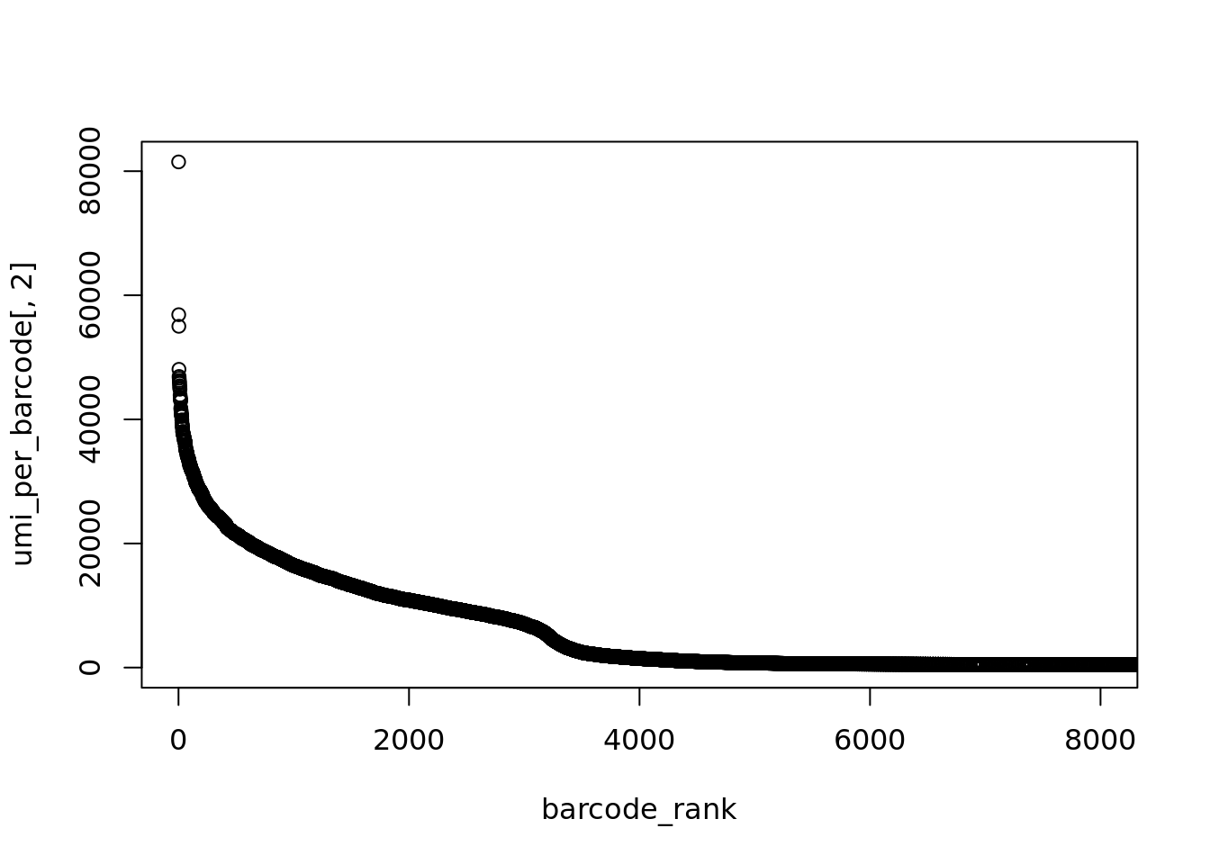
5.9.1 ‘Knee’ point
One of the most used methods use the total molecules (could be applied to total reads) per barcode and try to find a “break point” between bigger libraries which are cells + some background and smaller libraries assumed to be purely background. Let’s load some example simulated data which contain both large and small cells:
umi_per_barcode <- read.table("data/droplet_id_example_per_barcode.txt.gz")
truth <- read.delim("data/droplet_id_example_truth.gz", sep=",")
Exercise How many unique barcodes were detected? How many true cells are present in the data? To simplify calculations for this section exclude all barcodes with fewer than 10 total molecules.
Answer
One approach is to look for the inflection point where the total molecules per barcode suddenly drops:
Here we can see an roughly exponential curve of library sizes, so to make things simpler lets log-transform them.
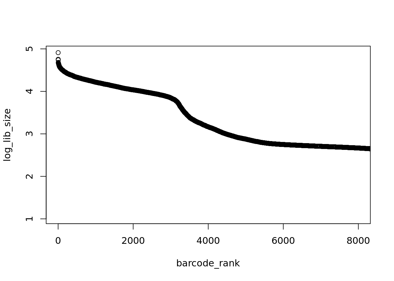
That’s better, the “knee” in the distribution is much more pronounced. We could manually estimate where the “knee” is but it much more reproducible to algorithmically identify this point.
# inflection point
o <- order(barcode_rank)
log_lib_size <- log_lib_size[o]
barcode_rank <- barcode_rank[o]

rawdiff <- diff(log_lib_size)/diff(barcode_rank)
inflection <- which(rawdiff == min(rawdiff[100:length(rawdiff)], na.rm=TRUE))

plot(barcode_rank, log_lib_size, xlim=c(1,8000))
abline(v=inflection, col="red", lwd=2)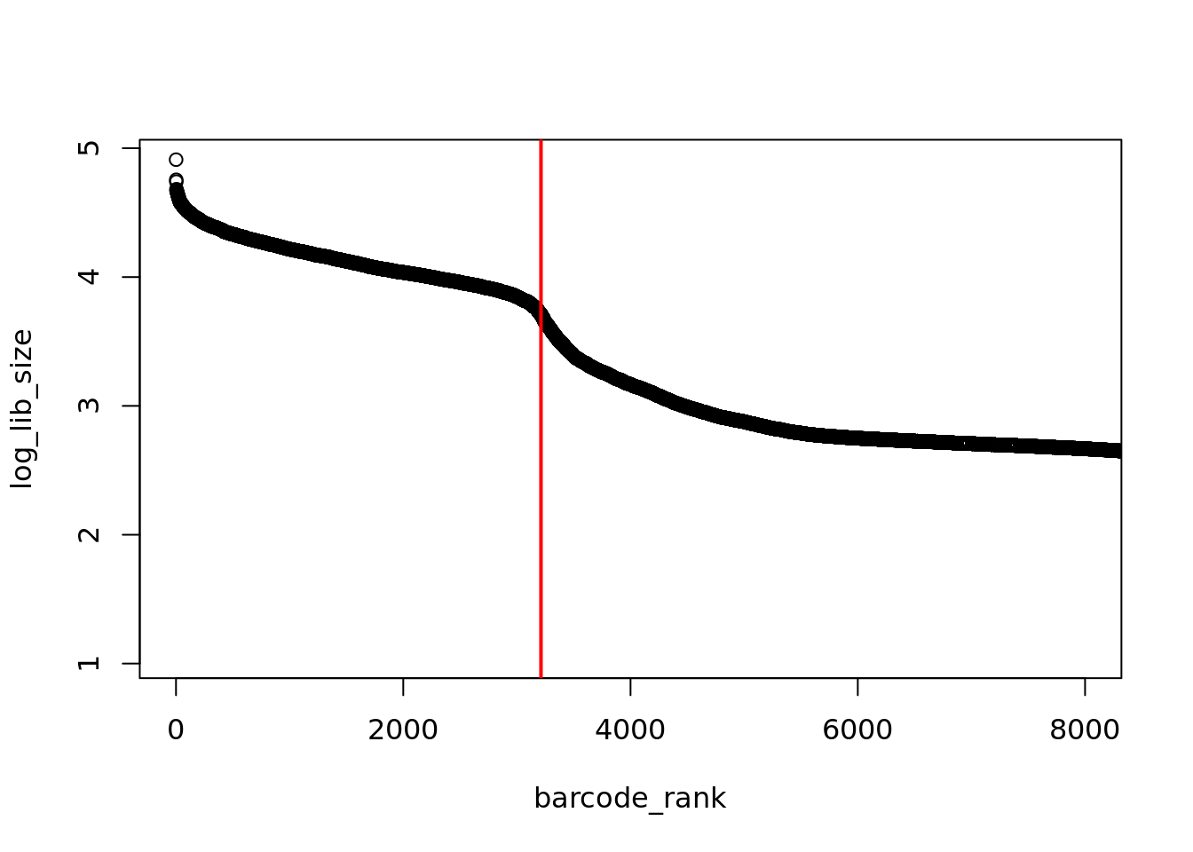
threshold <- 10^log_lib_size[inflection]

cells <- umi_per_barcode[umi_per_barcode[,2] > threshold,1]
TPR <- sum(cells %in% truth[,1])/length(cells)
Recall <- sum(cells %in% truth[,1])/length(truth[,1])
c(TPR, Recall)
## [1] 1.0000000 0.78317075.9.2 Mixture model
Another is to fix a mixture model and find where the higher and lower distributions intersect. However, data may not fit the assumed distributions very well:
## Loading required package: mixtools## mixtools package, version 1.1.0, Released 2017-03-10
## This package is based upon work supported by the National Science Foundation under Grant No. SES-0518772.## number of iterations= 43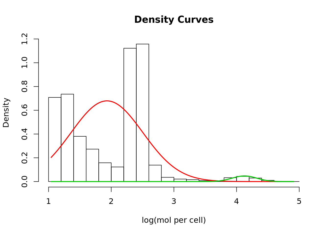
p1 <- dnorm(log_lib_size, mean=mix$mu[1], sd=mix$sigma[1])
p2 <- dnorm(log_lib_size, mean=mix$mu[2], sd=mix$sigma[2])
if (mix$mu[1] < mix$mu[2]) {
    split <- min(log_lib_size[p2 > p1])
} else {
    split <- min(log_lib_size[p1 > p2])
}
Exercise Identify cells using this split point and calculate the TPR and Recall.
Answer
5.9.3 Expected Number of Cells
A third method used by CellRanger V2, assumes a ~10-fold range of library sizes for real cells and estimates this range using the expected number of cells.
n_cells <- length(truth[,1])
# CellRanger v2
totals <- umi_per_barcode[,2]
totals <- sort(totals, decreasing = TRUE)
# 99th percentile of top n_cells divided by 10
thresh = totals[round(0.01*n_cells)]/10
plot(totals, xlim=c(1,8000))
abline(h=thresh, col="red", lwd=2)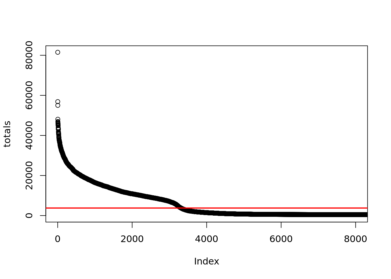 Exercise
Identify cells using this threshodl and calculate the TPR and Recall.
Exercise
Identify cells using this threshodl and calculate the TPR and Recall.
Answer
5.9.4 EmptyDroplets
Finally (EmptyDrops)[https://github.com/MarioniLab/DropletUtils] is what we recommend using in calling cell barcodes for droplet-based single-cell datasets. It should be noted that in cellranger count v3, EmptyDroptlet algoritms has been applied in their filtering for true cell barcode step.
Instead of trying to find a ‘threshold’ in UMIs counts for determining true cells, EmptyDroplet uses the full genes x cells molecule count matrix for all droplets and estimates the profile of
“background” RNA from those droplets with extremely low counts, then looks for
cells with gene-expression profiles which differ from the background.
This is combined with an inflection point method since background RNA often looks very similar to the expression profile of the largests cells in a population. As such EmptyDrops is the only method able to identify barcodes for very small cells in highly diverse samples.
Below we have provided code for how this method is currently run:
library("Matrix")
raw.counts <- readRDS("data/pancreas/muraro.rds")

library("DropletUtils")
example(write10xCounts, echo=FALSE)
dir.name <- tmpdir
list.files(dir.name)
sce <- read10xCounts(dir.name)
sce
my.counts <- DropletUtils:::simCounts()
br.out <- barcodeRanks(my.counts)

# Making a plot.
plot(br.out$rank, br.out$total, log="xy", xlab="Rank", ylab="Total")
o <- order(br.out$rank)
lines(br.out$rank[o], br.out$fitted[o], col="red")

abline(h=metadata(br.out)$knee, col="dodgerblue", lty=2)
abline(h=metadata(br.out)$inflection, col="forestgreen", lty=2)
legend("bottomleft", lty=2, col=c("dodgerblue", "forestgreen"),
    legend=c("knee", "inflection"))
# emptyDrops
set.seed(100)
e.out <- emptyDrops(my.counts)
is.cell <- e.out$FDR <= 0.01
sum(is.cell, na.rm=TRUE)

plot(e.out$Total, -e.out$LogProb, col=ifelse(is.cell, "red", "black"),
    xlab="Total UMI count", ylab="-Log Probability")

# plot(e.out$Total, -e.out$LogProb, col=ifelse(is.cell, "red", "black"),
#     xlab="Total UMI count", ylab="-Log Probability")
#
# cells <- colnames(raw.counts)[is.cell]
#
# TPR <- sum(cells %in% truth[,1])/length(cells)
# Recall <- sum(cells %in% truth[,1])/length(truth[,1])
# c(TPR, Recall)
References
Bray, Nicolas L, Harold Pimentel, Páll Melsted, and Lior Pachter. 2016. “Near-Optimal Probabilistic Rna-Seq Quantification.” Nat Biotechnol 34 (5): 525–27. https://doi.org/10.1038/nbt.3519.
Dobin, Alexander, Carrie A Davis, Felix Schlesinger, Jorg Drenkow, Chris Zaleski, Sonali Jha, Philippe Batut, Mark Chaisson, and Thomas R Gingeras. 2013. “STAR: Ultrafast Universal Rna-Seq Aligner.” Bioinformatics 29 (1): 15–21. https://doi.org/10.1093/bioinformatics/bts635.
Kolodziejczyk, Aleksandra A., Jong Kyoung Kim, Valentine Svensson, John C. Marioni, and Sarah A. Teichmann. 2015. “The Technology and Biology of Single-Cell RNA Sequencing.” Molecular Cell 58 (4). Elsevier BV: 610–20. https://doi.org/10.1016/j.molcel.2015.04.005.