2 Introduction to single-cell RNA-seq
2.1 Bulk RNA-seq
- A major breakthrough (replaced microarrays) in the late 00’s and has been widely used since
- Measures the average expression level for each gene across a large population of input cells
- Useful for comparative transcriptomics, e.g. samples of the same tissue from different species
- Useful for quantifying expression signatures from ensembles, e.g. in disease studies
- Insufficient for studying heterogeneous systems, e.g. early development studies, complex tissues (brain)
- Does not provide insights into the stochastic nature of gene expression
2.2 scRNA-seq
- A new technology, first publication by (Tang et al. 2009)
- Did not gain widespread popularity until ~2014 when new protocols and lower sequencing costs made it more accessible
- Measures the distribution of expression levels for each gene across a population of cells
- Allows to study new biological questions in which cell-specific changes in transcriptome are important, e.g. cell type identification, heterogeneity of cell responses, stochasticity of gene expression, inference of gene regulatory networks across the cells.
- Datasets range from \(10^2\) to \(10^6\) cells and increase in size every year
- Currently there are several different protocols in use, e.g. SMART-seq2 (Picelli et al. 2013), CELL-seq (Hashimshony et al. 2012) and Drop-seq (Macosko et al. 2015)
- There are also commercial platforms available, including the Fluidigm C1, Wafergen ICELL8 and the 10X Genomics Chromium
- Several computational analysis methods from bulk RNA-seq can be used
- In most cases computational analysis requires adaptation of the existing methods or development of new ones
2.3 Workflow
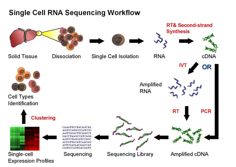
Figure 2.1: Single cell sequencing (taken from Wikipedia)
Overall, experimental scRNA-seq protocols are similar to the methods used for bulk RNA-seq. We will be discussing some of the most common approaches in the next chapter.
2.4 Computational Analysis
This course is concerned with the computational analysis of the data obtained from scRNA-seq experiments. The first steps (yellow) are general for any highthroughput sequencing data. Later steps (orange) require a mix of existing RNASeq analysis methods and novel methods to address the technical difference of scRNASeq. Finally the biological interpretation (blue) should be analyzed with methods specifically developed for scRNASeq.
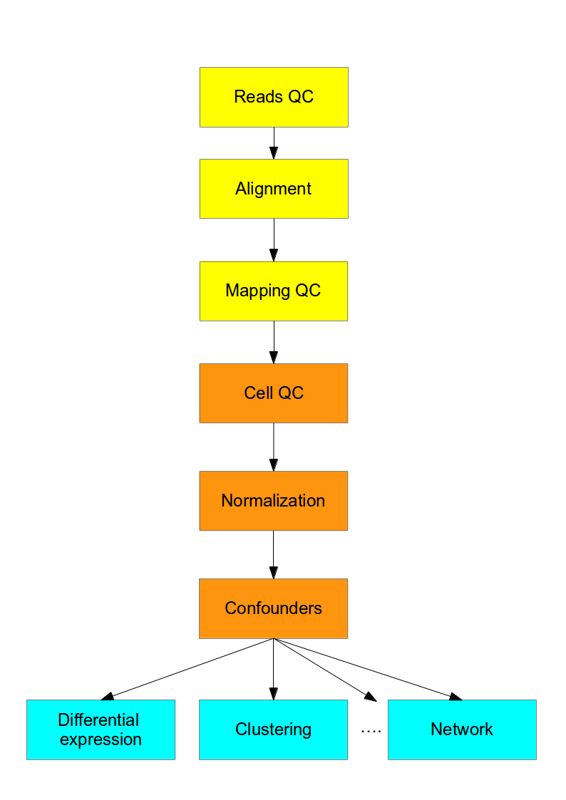
Figure 2.2: Flowchart of the scRNA-seq analysis
There are several reviews of the scRNA-seq analysis available including (Stegle, Teichmann, and Marioni 2015).
Today, there are also several different platforms available for carrying out one or more steps in the flowchart above. These include:
- Falco a single-cell RNA-seq processing framework on the cloud.
- SCONE (Single-Cell Overview of Normalized Expression), a package for single-cell RNA-seq data quality control and normalization.
- Seurat is an R package designed for QC, analysis, and exploration of single cell RNA-seq data.
- ASAP (Automated Single-cell Analysis Pipeline) is an interactive web-based platform for single-cell analysis.
- Bioconductor is a open-source, open-development software project for the analysis of high-throughput genomics data, including packages for the analysis of single-cell data.
2.5 Challenges
The main difference between bulk and single cell RNA-seq is that each sequencing library represents a single cell, instead of a population of cells. Therefore, significant attention has to be paid to comparison of the results from different cells (sequencing libraries). The main sources of discrepancy between the libraries are:
- Reverse transcription to convert RNA to cDNA is at best <30% efficient
- Amplification (up to 1 million fold)
- Gene ‘dropouts’ in which a gene is observed at a moderate expression level in one cell but is not detected in another cell (Kharchenko, Silberstein, and Scadden 2014); this can be due to technical factors (e.g. inefficient RT) or true biological variability across cells.
These discrepancies are introduced due to low starting amounts of transcripts since the RNA comes from one cell only. Improving the transcript capture efficiency and reducing the amplification bias are currently active areas of research. However, as we shall see in this course, it is possible to alleviate some of these issues through proper normalization and corrections and effective statistical models.
For the analyst, the characteristics of single-cell RNA-seq data lead to challenges in handling:
- Sparsity
- Variability
- Scalability
- Complexity
In this workshop we will present computational approaches that can allow us to face these challenges as we try to answer biological questions of interest from single-cell transcriptomic data.
2.6 Experimental methods
)](figures/moores-law.png)
Figure 2.3: Moore’s law in single cell transcriptomics (image taken from Svensson et al)
Development of new methods and protocols for scRNA-seq is currently a very active area of research, and several protocols have been published over the last few years. A non-comprehensive list includes:
- CEL-seq (Hashimshony et al. 2012)
- CEL-seq2 (Hashimshony et al. 2016)
- Drop-seq (Macosko et al. 2015)
- InDrop-seq (Klein et al. 2015)
- MARS-seq (Jaitin et al. 2014)
- SCRB-seq (Soumillon et al. 2014)
- Seq-well (Gierahn et al. 2017)
- Smart-seq (Picelli et al. 2014)
- Smart-seq2 (Picelli et al. 2014)
- SMARTer
- STRT-seq (Islam et al. 2013)
The methods can be categorized in different ways, but the two most important aspects are quantification and capture.
For quantification, there are two types, full-length and tag-based. The former tries to achieve a uniform read coverage of each transcript. By contrast, tag-based protocols only capture either the 5’- or 3’-end of each RNA. The choice of quantification method has important implications for what types of analyses the data can be used for. In theory, full-length protocols should provide an even coverage of transcripts, but as we shall see, there are often biases in the coverage. The main advantage of tag-based protocol is that they can be combined with unique molecular identifiers (UMIs) which can help improve the quantification (see chapter 2.8). On the other hand, being restricted to one end of the transcript may reduce the mappability and it also makes it harder to distinguish different isoforms (Archer et al. 2016).
The strategy used for capture determines throughput, how the cells can be selected as well as what kind of additional information besides the sequencing that can be obtained. The three most widely used options are microwell-, microfluidic- and droplet- based.
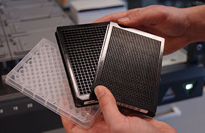
Figure 2.4: Image of microwell plates (image taken from Wikipedia)
For well-based platforms, cells are isolated using for example pipette or laser capture and placed in microfluidic wells. One advantage of well-based methods is that they can be combined with fluorescent activated cell sorting (FACS), making it possible to select cells based on surface markers. This strategy is thus very useful for situations when one wants to isolate a specific subset of cells for sequencing. Another advantage is that one can take pictures of the cells. The image provides an additional modality and a particularly useful application is to identify wells containg damaged cells or doublets. The main drawback of these methods is that they are often low-throughput and the amount of work required per cell may be considerable.
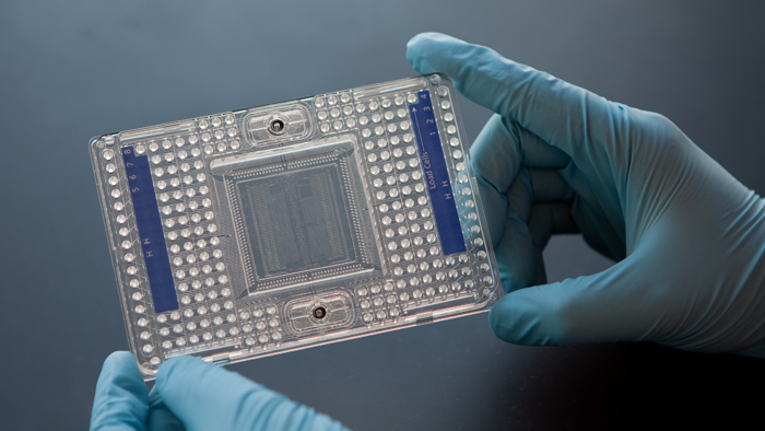
Figure 2.5: Image of a 96-well Fluidigm C1 chip (image taken from Fluidigm)
Microfluidic platforms, such as Fluidigm’s C1, provide a more integrated system for capturing cells and for carrying out the reactions necessary for the library preparations. Thus, they provide a higher throughput than microwell based platforms. Typically, only around 10% of cells are captured in a microfluidic platform and thus they are not appropriate if one is dealing with rare cell-types or very small amounts of input. Moreover, the chip is relatively expensive, but since reactions can be carried out in a smaller volume money can be saved on reagents.
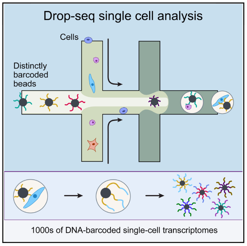
Figure 2.6: Schematic overview of the drop-seq method (Image taken from Macosko et al)
The idea behind droplet based methods is to encapsulate each individual cell inside a nanoliter droplet together with a bead. The bead is loaded with the enzymes required to construct the library. In particular, each bead contains a unique barcode which is attached to all of the reads originating from that cell. Thus, all of the droplets can be pooled, sequenced together and the reads can subsequently be assigned to the cell of origin based on the barcodes. Droplet platforms typically have the highest throughput since the library preparation costs are on the order of \(.05\) USD/cell. Instead, sequencing costs often become the limiting factor and a typical experiment the coverage is low with only a few thousand different transcripts detected (Ziegenhain et al. 2017).
2.7 What platform to use for my experiment?
The most suitable platform depends on the biological question at hand. For example, if one is interested in characterizing the composition of a tissue, then a droplet-based method which will allow a very large number of cells to be captured is likely to be the most appropriate. On the other hand, if one is interesting in characterizing a rare cell-population for which there is a known surface marker, then it is probably best to enrich using FACS and then sequence a smaller number of cells.
Clearly, full-length transcript quantification will be more appropriate if one is interested in studying different isoforms since tagged protocols are much more limited. By contrast, UMIs can only be used with tagged protocols and they can facilitate gene-level quantification.
Two recent studies from the Enard group (Ziegenhain et al. 2017) and the Teichmann group (Svensson et al. 2017) have compared several different protocols. In their study, Ziegenhain et al compared five different protocols on the same sample of mouse embryonic stem cells (mESCs). By controlling for the number of cells as well as the sequencing depth, the authors were able to directly compare the sensitivity, noise-levels and costs of the different protocols. One example of their conclusions is illustrated in the figure below which shows the number of genes detected (for a given detection threshold) for the different methods. As you can see, there is almost a two-fold difference between drop-seq and Smart-seq2, suggesting that the choice of protocol can have a major impact on the study
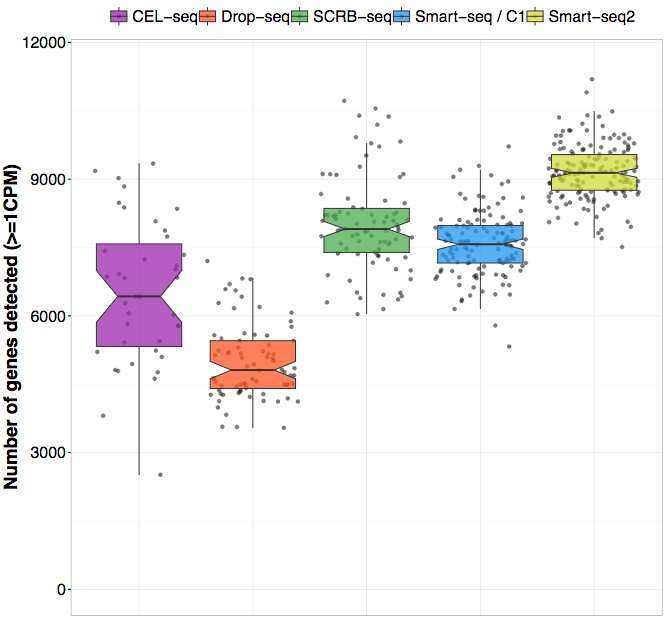
Figure 2.7: Enard group study
Svensson et al take a different approach by using synthetic transcripts (spike-ins, more about these later) with known concentrations to measure the accuracy and sensitivity of different protocols. Comparing a wide range of studies, they also reported substantial differences between the protocols.
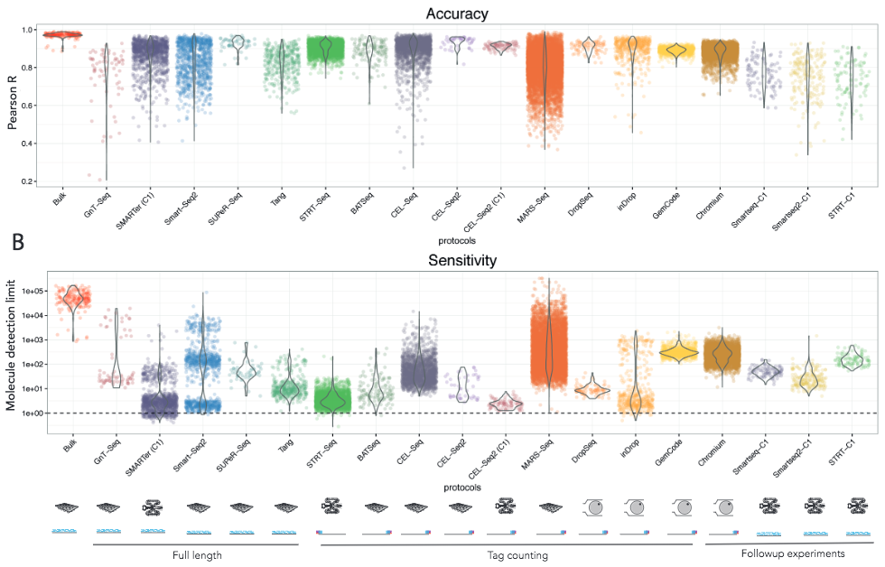
Figure 2.8: Teichmann group study
As protocols are developed and computational methods for quantifying the technical noise are improved, it is likely that future studies will help us gain further insights regarding the strengths of the different methods. These comparative studies are helpful not only for helping researchers decide which protocol to use, but also for developing new methods as the benchmarking makes it possible to determine what strategies are the most useful ones.
2.8 Unique Molecular Identifiers (UMIs)
Thanks to Andreas Buness from EMBL Monterotondo for collaboration on this section.
2.8.1 Introduction
Unique Molecular Identifiers are short (4-10bp) random barcodes added to transcripts during reverse-transcription. They enable sequencing reads to be assigned to individual transcript molecules and thus the removal of amplification noise and biases from scRNASeq data.
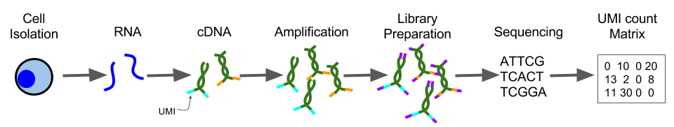
Figure 2.9: UMI sequencing protocol
When sequencing UMI containing data, techniques are used to specifically sequence only the end of the transcript containing the UMI (usually the 3’ end).
2.8.2 Mapping Barcodes
Since the number of unique barcodes (\(4^N\), where \(N\) is the length of UMI) is much smaller than the total number of molecules per cell (~\(10^6\)), each barcode will typically be assigned to multiple transcripts. Hence, to identify unique molecules both barcode and mapping location (transcript) must be used. The first step is to map UMI reads, for which we recommend using STAR since it is fast and outputs good quality BAM-alignments. Moreover, mapping locations can be useful for eg. identifying poorly-annotated 3’ UTRs of transcripts.
UMI-sequencing typically consists of paired-end reads where one read from each pair captures the cell and UMI barcodes while the other read consists of exonic sequence from the transcript (Figure 2.10). Note that trimming and/or filtering to remove reads containing poly-A sequence is recommended to avoid erors due to these read mapping to genes/transcripts with internal poly-A/poly-T sequences.
After processing the reads from a UMI experiment, the following conventions are often used:
The UMI is added to the read name of the other paired read.
- Reads are sorted into separate files by cell barcode
- For extremely large, shallow datasets, the cell barcode may be added to the read name as well to reduce the number of files.
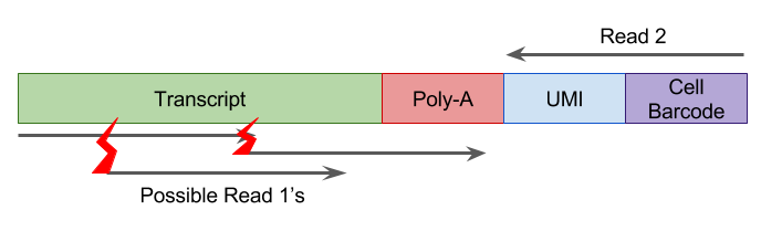
Figure 2.10: UMI sequencing reads, red lightning bolts represent different fragmentation locations
2.8.3 Counting Barcodes
In theory, every unique UMI-transcript pair should represent all reads originating from a single RNA molecule. However, in practice this is frequently not the case and the most common reasons are:
- Different UMI does not necessarily mean different molecule
- Due to PCR or sequencing errors, base-pair substitution events can result in new UMI sequences. Longer UMIs give more opportunity for errors to arise and based on estimates from cell barcodes we expect 7-10% of 10bp UMIs to contain at least one error. If not corrected for, this type of error will result in an overestimate of the number of transcripts.
- Different transcript does not necessarily mean different molecule
- Mapping errors and/or multimapping reads may result in some UMIs being assigned to the wrong gene/transcript. This type of error will also result in an overestimate of the number of transcripts.
- Same UMI does not necessarily mean same molecule
- Biases in UMI frequency and short UMIs can result in the same UMI being attached to different mRNA molecules from the same gene. Thus, the number of transcripts may be underestimated.
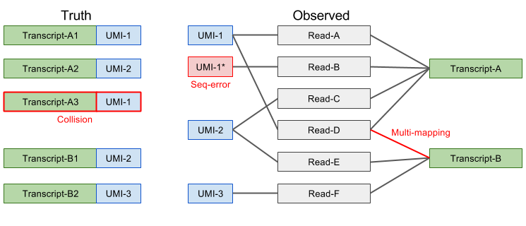
Figure 2.11: Potential Errors in UMIs
2.8.4 Correcting for Errors
How to best account for errors in UMIs remains an active area of research. The best approaches that we are aware of for resolving the issues mentioned above are:
UMI-tools’ directional-adjacency method implements a procedure which considers both the number of mismatches and the relative frequency of similar UMIs to identify likely PCR/sequencing errors.
Currently an open question. The problem may be mitigated by removing UMIs with few reads to support their association with a particular transcript, or by removing all multi-mapping reads.
Simple saturation (aka “collision probability”) correction proposed by Grun, Kester and van Oudenaarden (2014) to estimate the true number of molecules \(M\):
\[M \approx -N*log(1 - \frac{n}{N})\] where N = total number of unique UMI barcodes and n = number of observed barcodes.
An important caveat of this method is that it assumes that all UMIs are equally frequent. In most cases this is incorrect, since there is often a bias related to the GC content.
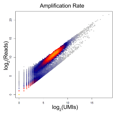
Figure 2.12: Per gene amplification rate
Determining how to best process and use UMIs is currently an active area of research in the bioinformatics community. We are aware of several methods that have recently been developed, including:
2.8.5 Downstream Analysis
Current UMI platforms (DropSeq, InDrop, ICell8) exhibit low and highly variable capture efficiency as shown in the figure below.
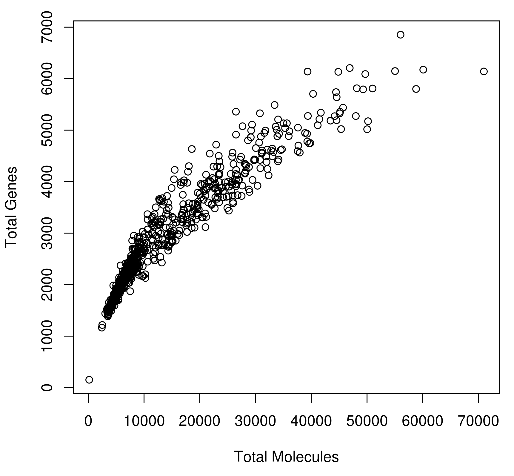
Figure 2.13: Variability in Capture Efficiency
This variability can introduce strong biases and it needs to be considered in downstream analysis. Recent analyses often pool cells/genes together based on cell-type or biological pathway to increase the power. Robust statistical analyses of this data is still an open research question and it remains to be determined how to best adjust for biases.
Exercise 1 We have provided you with UMI counts and read counts from induced pluripotent stem cells generated from three different individuals (Tung et al. 2017) (see: Chapter 6.1 for details of this dataset).
umi_counts <- read.table("data/tung/molecules.txt", sep = "\t")
read_counts <- read.table("data/tung/reads.txt", sep = "\t")
Using this data:
Plot the variability in capture efficiency
Determine the amplification rate: average number of reads per UMI.
References
Archer, Nathan, Mark D. Walsh, Vahid Shahrezaei, and Daniel Hebenstreit. 2016. “Modeling Enzyme Processivity Reveals That RNA-Seq Libraries Are Biased in Characteristic and Correctable Ways.” Cell Systems 3 (5). Elsevier BV: 467–479.e12. https://doi.org/10.1016/j.cels.2016.10.012.
Gierahn, Todd M, Marc H Wadsworth 2nd, Travis K Hughes, Bryan D Bryson, Andrew Butler, Rahul Satija, Sarah Fortune, J Christopher Love, and Alex K Shalek. 2017. “Seq-Well: Portable, Low-Cost RNA Sequencing of Single Cells at High Throughput.” Nat. Methods 14 (4): 395–98.
Hashimshony, Tamar, Naftalie Senderovich, Gal Avital, Agnes Klochendler, Yaron de Leeuw, Leon Anavy, Dave Gennert, et al. 2016. “CEL-Seq2: Sensitive Highly-Multiplexed Single-Cell RNA-Seq.” Genome Biol 17 (1). Springer Nature. https://doi.org/10.1186/s13059-016-0938-8.
Hashimshony, Tamar, Florian Wagner, Noa Sher, and Itai Yanai. 2012. “CEL-Seq: Single-cell RNA-Seq by Multiplexed Linear Amplification.” Cell Reports 2 (3). Elsevier BV: 666–73. https://doi.org/10.1016/j.celrep.2012.08.003.
Islam, Saiful, Amit Zeisel, Simon Joost, Gioele La Manno, Pawel Zajac, Maria Kasper, Peter Lönnerberg, and Sten Linnarsson. 2013. “Quantitative Single-Cell RNA-Seq with Unique Molecular Identifiers.” Nat Meth 11 (2). Springer Nature: 163–66. https://doi.org/10.1038/nmeth.2772.
Jaitin, Diego Adhemar, Ephraim Kenigsberg, Hadas Keren-Shaul, Naama Elefant, Franziska Paul, Irina Zaretsky, Alexander Mildner, et al. 2014. “Massively Parallel Single-Cell RNA-seq for Marker-Free Decomposition of Tissues into Cell Types.” Science 343 (6172): 776–79.
Kharchenko, Peter V, Lev Silberstein, and David T Scadden. 2014. “Bayesian Approach to Single-Cell Differential Expression Analysis.” Nat Meth 11 (7). Springer Nature: 740–42. https://doi.org/10.1038/nmeth.2967.
Klein, Allon M., Linas Mazutis, Ilke Akartuna, Naren Tallapragada, Adrian Veres, Victor Li, Leonid Peshkin, David A. Weitz, and Marc W. Kirschner. 2015. “Droplet Barcoding for Single-Cell Transcriptomics Applied to Embryonic Stem Cells.” Cell 161 (5). Elsevier BV: 1187–1201. https://doi.org/10.1016/j.cell.2015.04.044.
Macosko, Evan Z., Anindita Basu, Rahul Satija, James Nemesh, Karthik Shekhar, Melissa Goldman, Itay Tirosh, et al. 2015. “Highly Parallel Genome-Wide Expression Profiling of Individual Cells Using Nanoliter Droplets.” Cell 161 (5). Elsevier BV: 1202–14. https://doi.org/10.1016/j.cell.2015.05.002.
Picelli, Simone, Åsa K Björklund, Omid R Faridani, Sven Sagasser, Gösta Winberg, and Rickard Sandberg. 2013. “Smart-Seq2 for Sensitive Full-Length Transcriptome Profiling in Single Cells.” Nat Meth 10 (11). Springer Nature: 1096–8. https://doi.org/10.1038/nmeth.2639.
Picelli, Simone, Omid R Faridani, Asa K Björklund, Gösta Winberg, Sven Sagasser, and Rickard Sandberg. 2014. “Full-Length RNA-seq from Single Cells Using Smart-Seq2.” Nat. Protoc. 9 (1): 171–81.
Soumillon, Magali, Davide Cacchiarelli, Stefan Semrau, Alexander van Oudenaarden, and Tarjei S Mikkelsen. 2014. “Characterization of Directed Differentiation by High-Throughput Single-Cell RNA-Seq.” bioRxiv, March, 003236.
Stegle, Oliver, Sarah A. Teichmann, and John C. Marioni. 2015. “Computational and Analytical Challenges in Single-Cell Transcriptomics.” Nat Rev Genet 16 (3). Springer Nature: 133–45. https://doi.org/10.1038/nrg3833.
Svensson, Valentine, Kedar Nath Natarajan, Lam-Ha Ly, Ricardo J Miragaia, Charlotte Labalette, Iain C Macaulay, Ana Cvejic, and Sarah A Teichmann. 2017. “Power Analysis of Single-Cell RNA-Sequencing Experiments.” Nat Meth 14 (4). Springer Nature: 381–87. https://doi.org/10.1038/nmeth.4220.
Tang, Fuchou, Catalin Barbacioru, Yangzhou Wang, Ellen Nordman, Clarence Lee, Nanlan Xu, Xiaohui Wang, et al. 2009. “mRNA-Seq Whole-Transcriptome Analysis of a Single Cell.” Nat Meth 6 (5). Springer Nature: 377–82. https://doi.org/10.1038/nmeth.1315.
Tung, Po-Yuan, John D. Blischak, Chiaowen Joyce Hsiao, David A. Knowles, Jonathan E. Burnett, Jonathan K. Pritchard, and Yoav Gilad. 2017. “Batch Effects and the Effective Design of Single-Cell Gene Expression Studies.” Sci. Rep. 7 (January). Springer Nature: 39921. https://doi.org/10.1038/srep39921.
Ziegenhain, Christoph, Beate Vieth, Swati Parekh, Björn Reinius, Amy Guillaumet-Adkins, Martha Smets, Heinrich Leonhardt, Holger Heyn, Ines Hellmann, and Wolfgang Enard. 2017. “Comparative Analysis of Single-Cell RNA Sequencing Methods.” Molecular Cell 65 (4). Elsevier BV: 631–643.e4. https://doi.org/10.1016/j.molcel.2017.01.023.