9 Latent spaces
In many cases we may like to think of cells sitting in a low-dimensional, “latent” space that captures relationships between cells more intuitively than the very high-dimensional gene expression space.
library(scater)
library(SingleCellExperiment)
library(glmpca)
library(ggplot2)
library(Polychrome)
library(slalom)
9.1 Dimensionality reduction
Why?
- Reduce Curse of Dimensionality problems
- Increase storage and computational efficiency
- Visualize Data in 2D or 3D
Difficulty: Need to decide how many dimension to keep.
9.1.1 PCA: Principal component analysis
9.1.1.1 (traditional) PCA
PCA is a linear feature extraction technique. It performs a linear mapping of the data to a lower-dimensional space in such a way that the variance of the data in the low-dimensional representation is maximized. It does so by calculating the eigenvectors from the covariance matrix. The eigenvectors that correspond to the largest eigenvalues (the principal components) are used to reconstruct a significant fraction of the variance of the original data.
In simpler terms, PCA combines your input features in a specific way that you can drop the least important feature while still retaining the most valuable parts of all of the features. As an added benefit, each of the new features or components created after PCA are all independent of one another.
9.1.1.1.1 Basic ideas of PCA
- Idea1: Dropping dimensions = Projection onto lower dimensional space
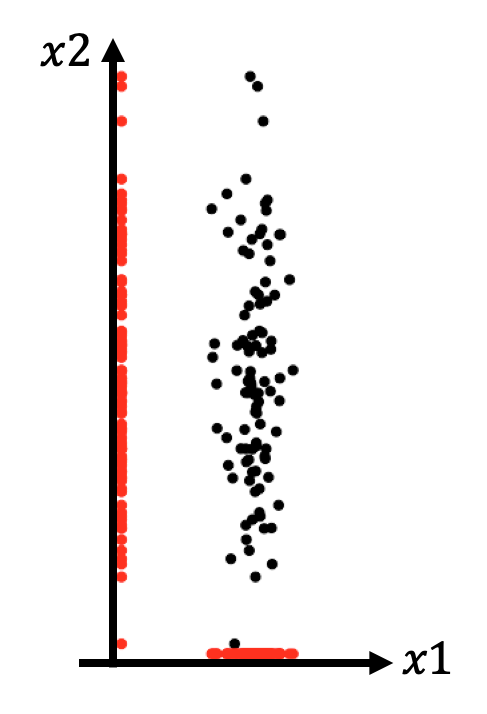
Which dimension should we keep?
- Idea2: more variantion = more information
9.1.1.1.2 Steps of PCA
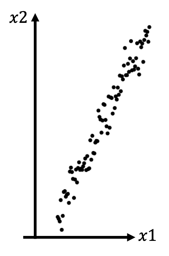
- Step1: Rotation
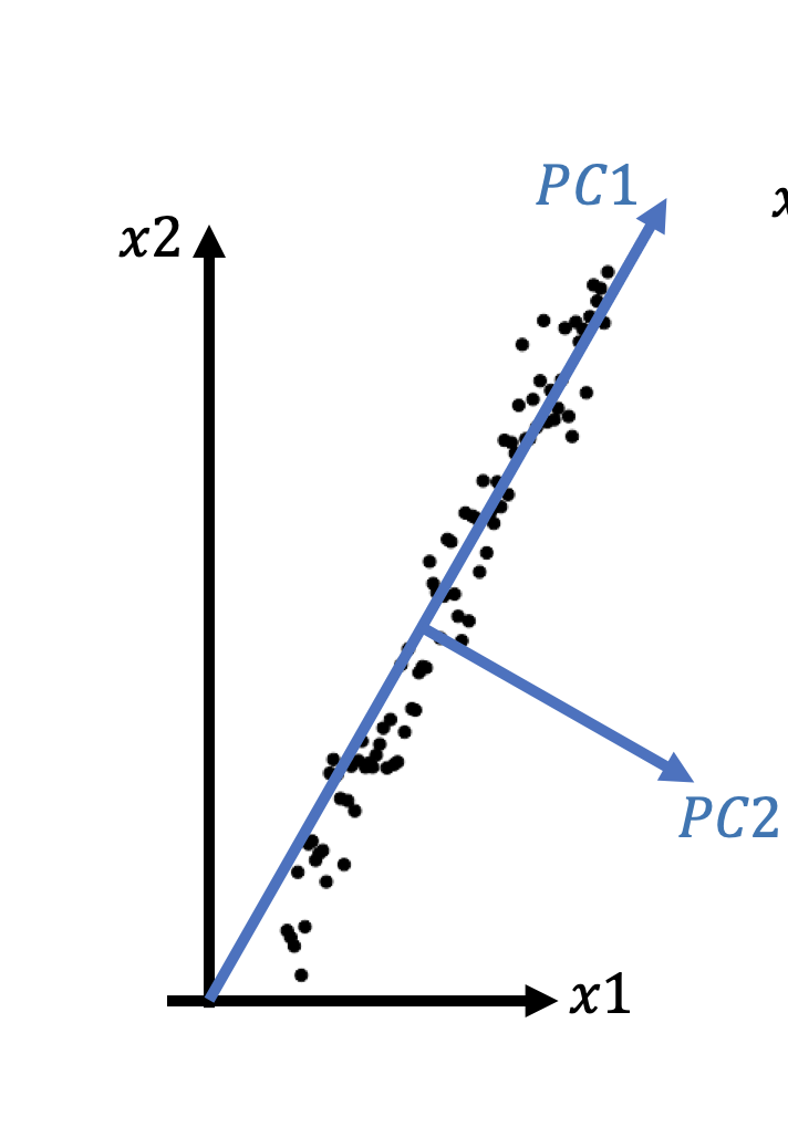
We want a set of axises (called Principle Components) that satisfies:
-The 1st axis points to the direction where variantion is maximized, and so on
-They are orthogonal to each other
It can be shown that the eigen vectors of the covariance matrix satisfy these conditions, and the eigen vector according to the largest eigen value accounts for the most variation.
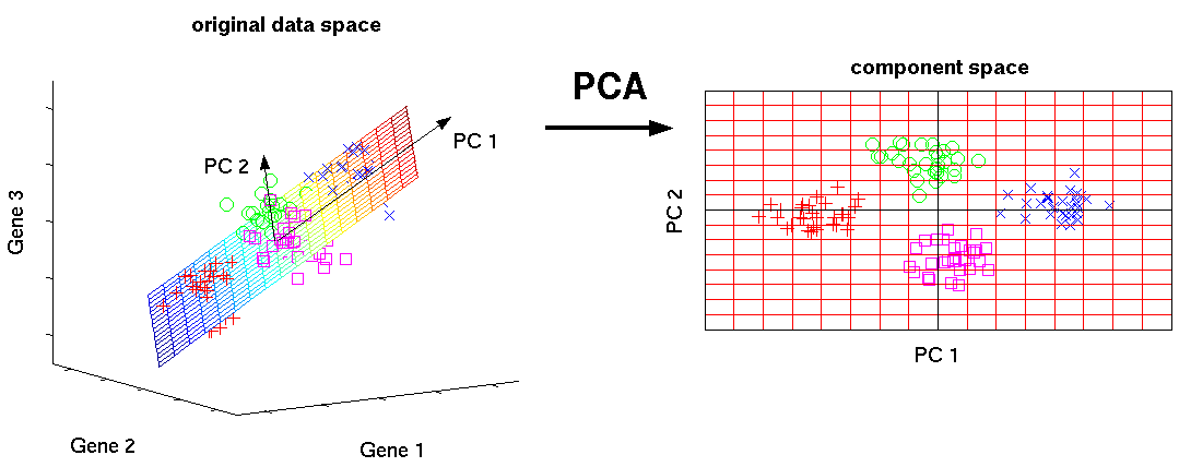
- Step2: Projection (3-dimesion \(\rightarrow\) 2-dimension)
9.1.1.1.3 An example of PCA
deng <- readRDS("data/deng/deng-reads.rds")
my_color1 <- createPalette(6, c("#010101", "#ff0000"), M=1000)
names(my_color1) <- unique(as.character(deng$cell_type1))
my_color2 <- createPalette(10, c("#010101", "#ff0000"), M=1000)
names(my_color2) <- unique(as.character(deng$cell_type2))
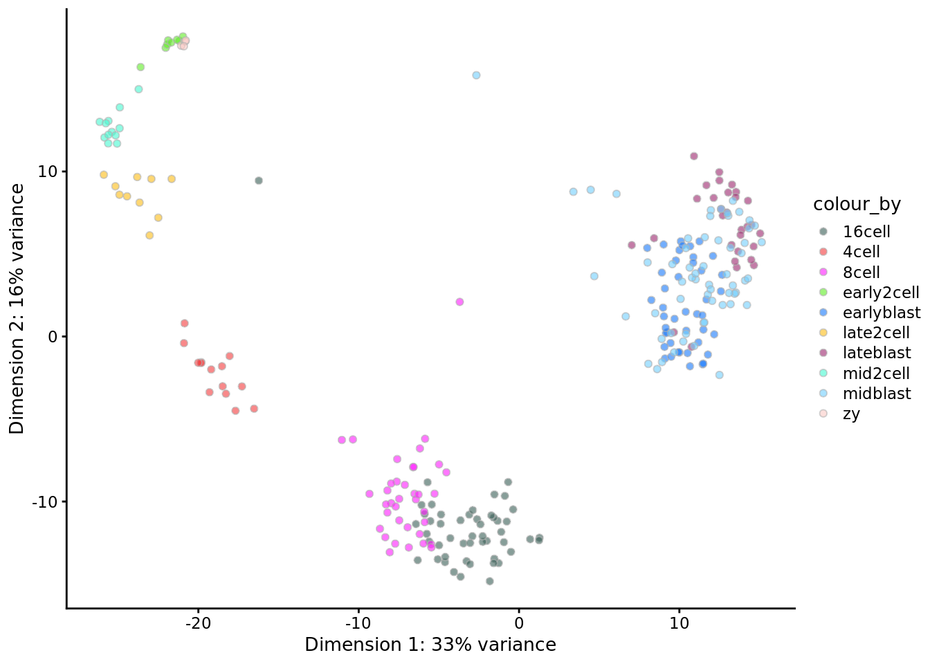
deng <- runPCA(deng, ncomponents = 2)
plotPCA(deng, colour_by = "cell_type1") +
scale_fill_manual(values = my_color1)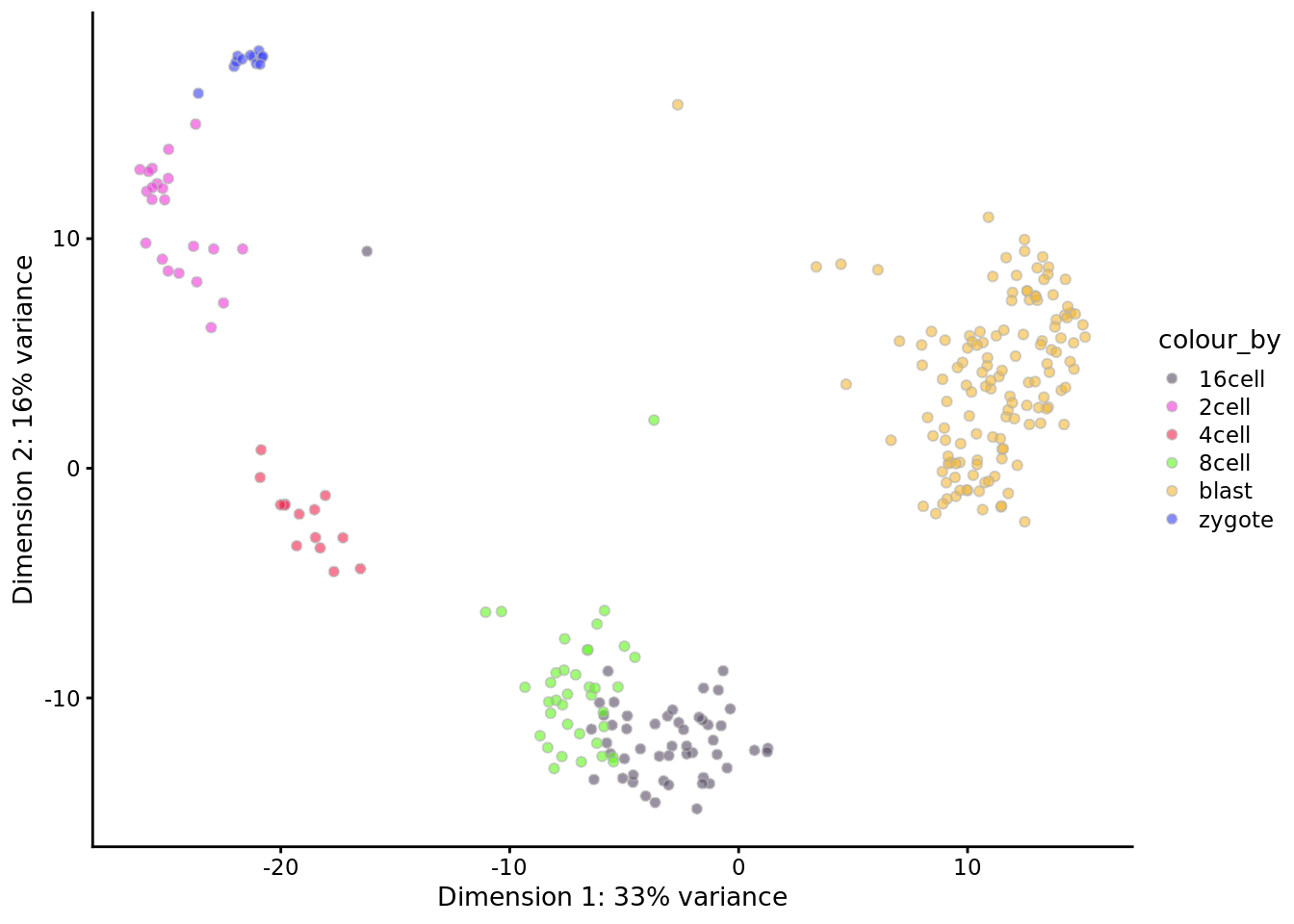
9.1.1.1.4 Advantages and limits of PCA:
Advantages: fast, easy to use and intuitive.
Limits:
Can lead to local inconsistency, i.e. far away points can become nearest neighbours.
- It is a linear projection, like casting a shadow, meaning it can’t capture
non-linear dependencies. For instance, PCA would not be able to “unroll” the
following structure.

9.1.1.2 GLM-PCA
(Collins, Dasgupta, and Schapire 2002) (Townes et al. 2019)
GLM-PCA is a generalized version of the traditional PCA.
The traditional PCA implicitly imposes an assumption of Gaussian distribution. The purpose of GLM-PCA is to loosen this condition to accommodate other distributions of the exponential family.
Why does PCA assume a Gaussian distribution?
Let \(x_1, \dots, x_n \in \mathcal{R}^d\) be the \(d\)-dimensional data observed.
PCA is looking for their projections onto a subspace: \(u_1, \dots, u_n\),
such that \(\sum_{i = 1}^n \Vert x_i - u_i\Vert^2\) is minimized.
This objective function can be interpretated in two ways:
Interpretation 1: the variance of the projections/principal components: \(\sum_{i} \Vert u_i \Vert ^2\), if the data is centered at the origin (\(\sum_{i} x_i = 0\));
Interpretation 2: Each point \(x_i\) is thought of as a random draw from a probability distribution centered at \(u_i\).
If we take this probability as a unit Gaussian, that is \(x_i \sim N(u_i, 1)\), then the likelihood is
\(\prod_{i = 1}^n \exp (- \Vert x_i - u_i\Vert^2)\), and the negative log likelihood is exactly the objective function.
This assumption is often inappropriate for non-Gaussian distributed data, for example discrete data.
Therefore, GLM-PCA generalizes the Gaussian likelihood into a likelihood of any exponential-family distribution, and applies appropriate link functions to \(u_i\)’s in the same as a GLM does to non-Gaussian responses.
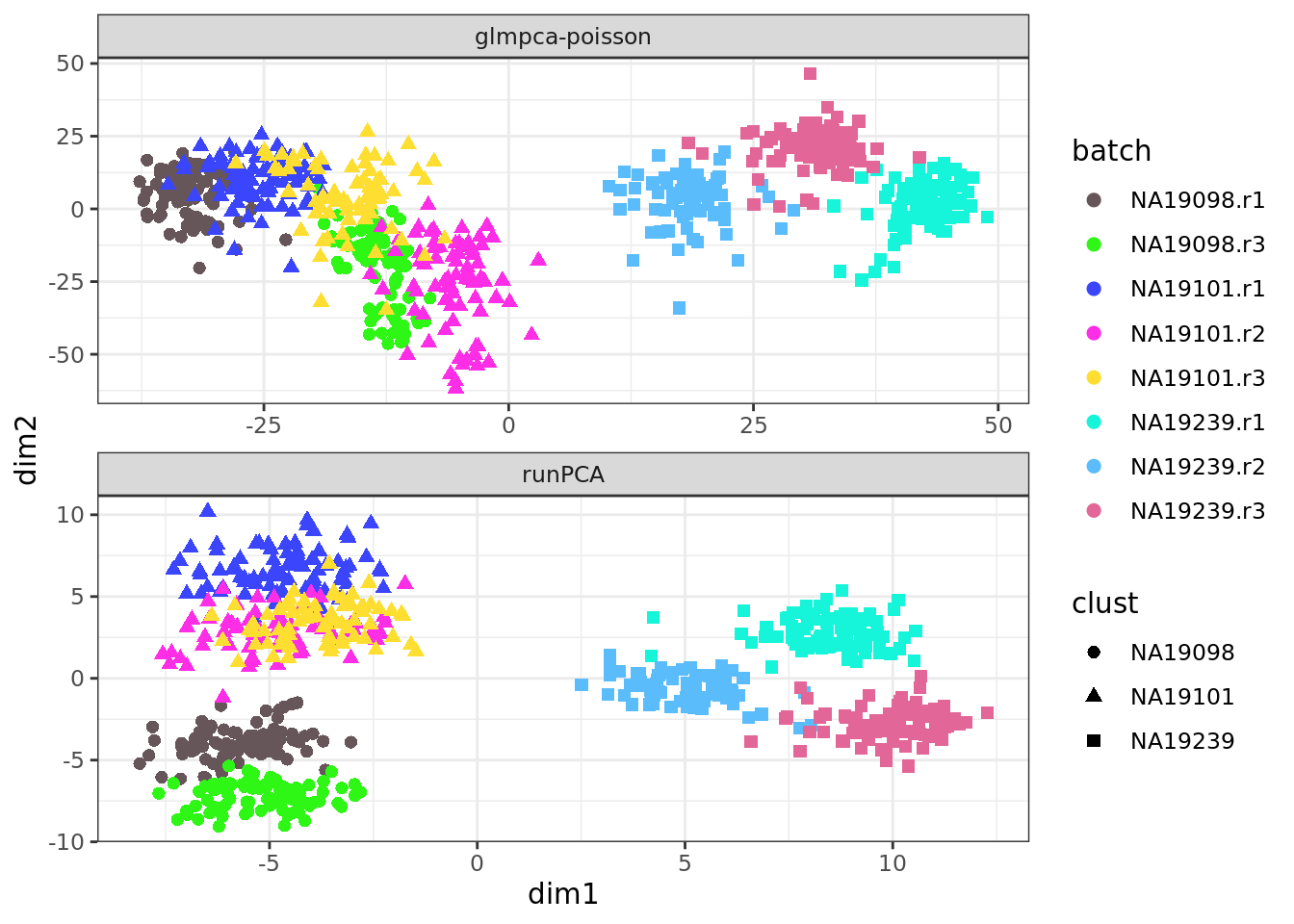
The following example compares GLM-PCA with Poisson marginals to the
traditional PCA, which is identical to the result from plotPCA.
## GLM-PCA
Y <- assay(deng, "counts")
Y <- Y[rowSums(Y) > 0, ]
system.time(res1 <- glmpca(Y, L=2, fam="poi", verbose=TRUE))
## user system elapsed
## 84.147 22.275 106.448pd1 <- data.frame(res1$factors, dimreduce="glmpca-poisson", clust = factor(deng$cell_type2))
## traditional PCA
pd2 <- data.frame(reducedDim(deng, "PCA"), dimreduce="runPCA", clust = factor(deng$cell_type2))
colnames(pd2) <- colnames(pd1)
## plot
pd <- rbind(pd1, pd2)
ggplot(pd, aes(x = dim1, y = dim2, colour = clust)) +
geom_point(size=2) +
facet_wrap(~dimreduce, scales="free", nrow=3) +
scale_color_manual(values = my_color2) +
theme_bw()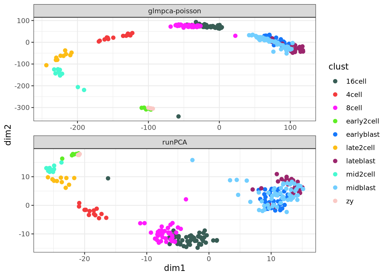
Let us compare GLM-PCA and standard PCA (using normalized log-counts data) on the Tung data, before cells have been QC’d.
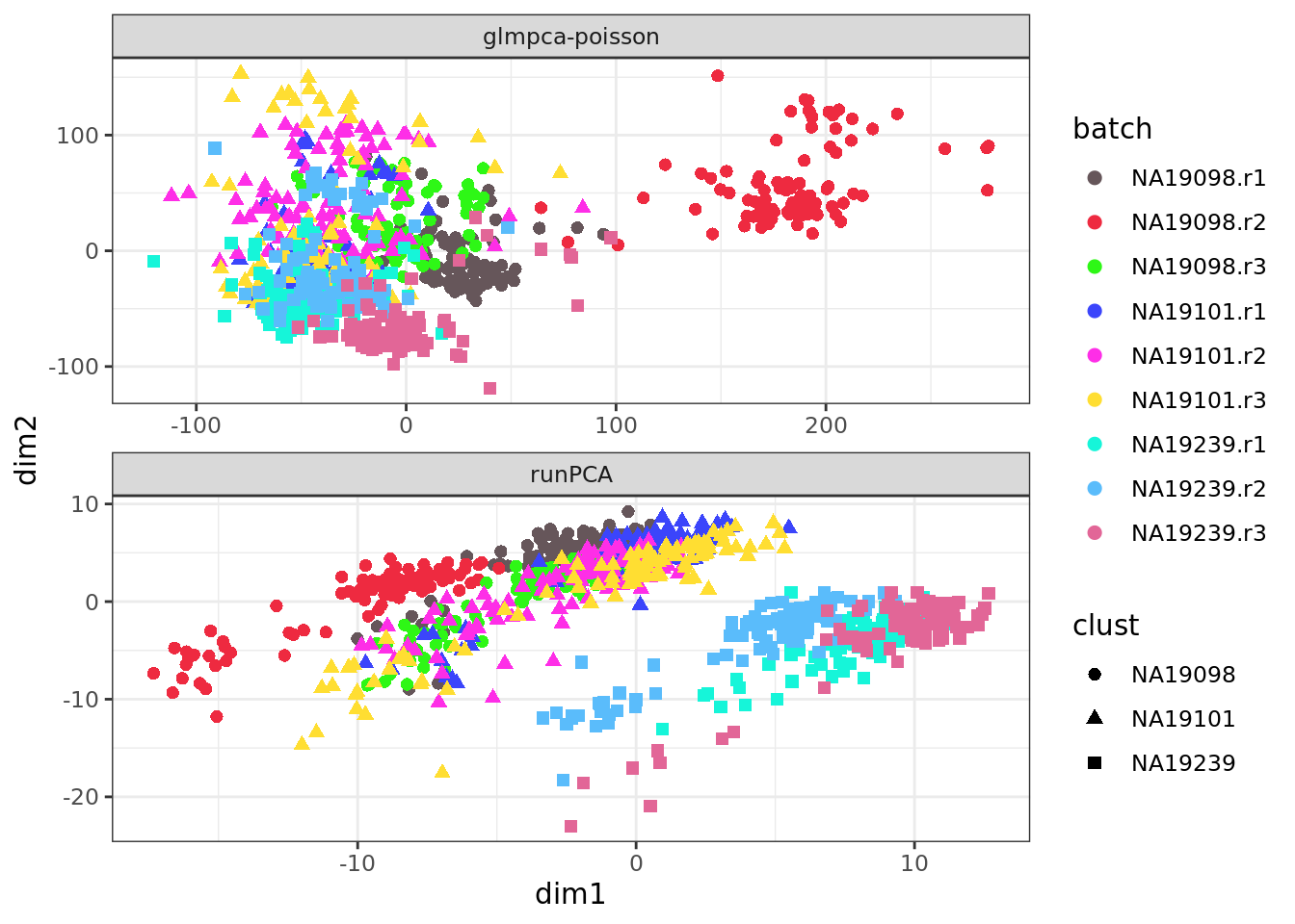
Repeat these plots with the QC’d Tung data.
9.1.2 tSNE: t-Distributed Stochastic Neighbor Embedding
t-SNE (Maaten and Hinton 2008) is an advanced version of the original SNE algorithm. (Hinton and Roweis 2003)
9.1.2.1 Motivation
The weakness of PCA is the motivation behind the SNE algorithm.
PCA focuses on global covariance structrue, which lead to local inconsistency.
SNE aims to preserve local strucutrue, or preserving the relationships among data points (ie. similar points remain similar; distinct points remain distinct).Unlike PCA, SNE is not limited to linear projections, which makes it suited to all sorts of datasets, including the swiss-roll data we have seen above.
t-SNE solves the crowding issue of the original SNE.
9.1.2.2 original SNE
SNE minimizes the divergence between two distributions: a distribution that measures pairwise similarities of the input objects and a distribution that measures pairwise similarities of the corresponding low-dimensional points in the embedding.
Goal: preserve neighbourhoods.
Soft neighbourhood:
For each data point \(x_i\), the \(i\rightarrow j\) probability is the probability that point \(x_i\) chooses \(x_j\) as its neighbour: \(p_{j|i} \propto \exp(-\Vert x_i - x_j \Vert^2/2\delta^2)\).
(This can be thought of as the probability of \(x_j\) in \(N(x_i, \delta)\))\(\Vert x_i - x_j \Vert^2\) is the Euclidean distance:
The closer \(x_i\) and \(x_j\) are, the larger \(p_{j|i}\) is.- \(\delta^2\) denotes the vairance, it sets the size of the neighbourhood.
Very low \(\Rightarrow\) all the probability is in the nearest neighbour
Very high \(\Rightarrow\) uniform weights
We generally want \(\delta^2\) to be small for points in densely populated areas and large for sparse areas, so that the number of neighbours of all data points are roughly the same. It is computed with a user specified parameter (perplexity) which indicates the effective number of neighbours for a data point.
Similarity matrix
Collect \(p_{j|i}\) for all data points into a matrix, then this matrix preserves the key information of the local neighbourhood structure.
How SNE works:
Given high-dimensional data \(X = \{x_1, \dots, x_n \in \mathcal{R}^d \}\), obtain the similarity matrix \(P\);
Let \(Y =\{y_1, \dots, y_n \in \mathcal{R}^2\}\) be a 2-dimensional data, the coordinates for visualization. Obtain a smilarity matrix of \(Y\), denoted as \(Q\), in the same way as \(X\), except that \(\delta^2\) is fixed at 1/2.
Look for \(Y\) such that \(Q\) is as similar to \(P\) as possible.
Measurement of how similar two distributions is: Kullback-Leibler divergence
(The definition of this cost function and the optimization procedure are out of the scope of this course)
9.1.2.3 t-SNE
The motivation of t-SNE is to solve one of the main issues of SNE, the crowding problem.
- Crowding problem:
In high dimension we have more room, points can have a lot of different neighbours that are far apart from each other. But in low dimensions, we don’t have enough room to accommodate all neighbours. Forexample, in 2D a point can have a few neighbors at distance one all far from each other - what happens when we embed in 1D?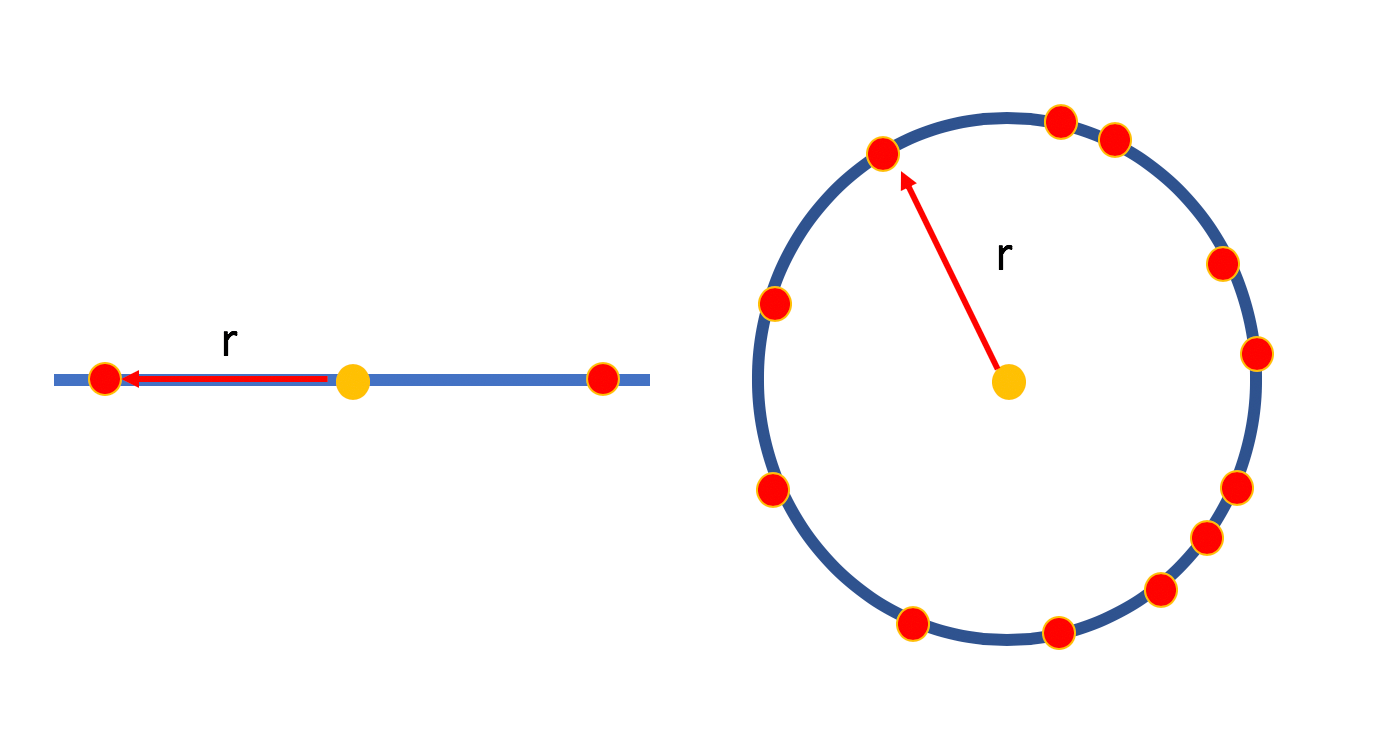
- Solution:
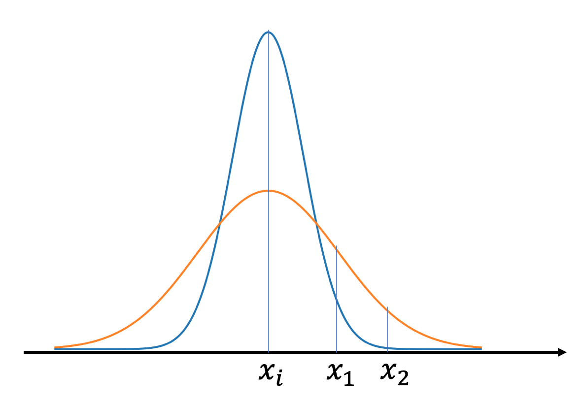
Change the distribution of the low-dimensional data \(Q\) into a student-t distribution.
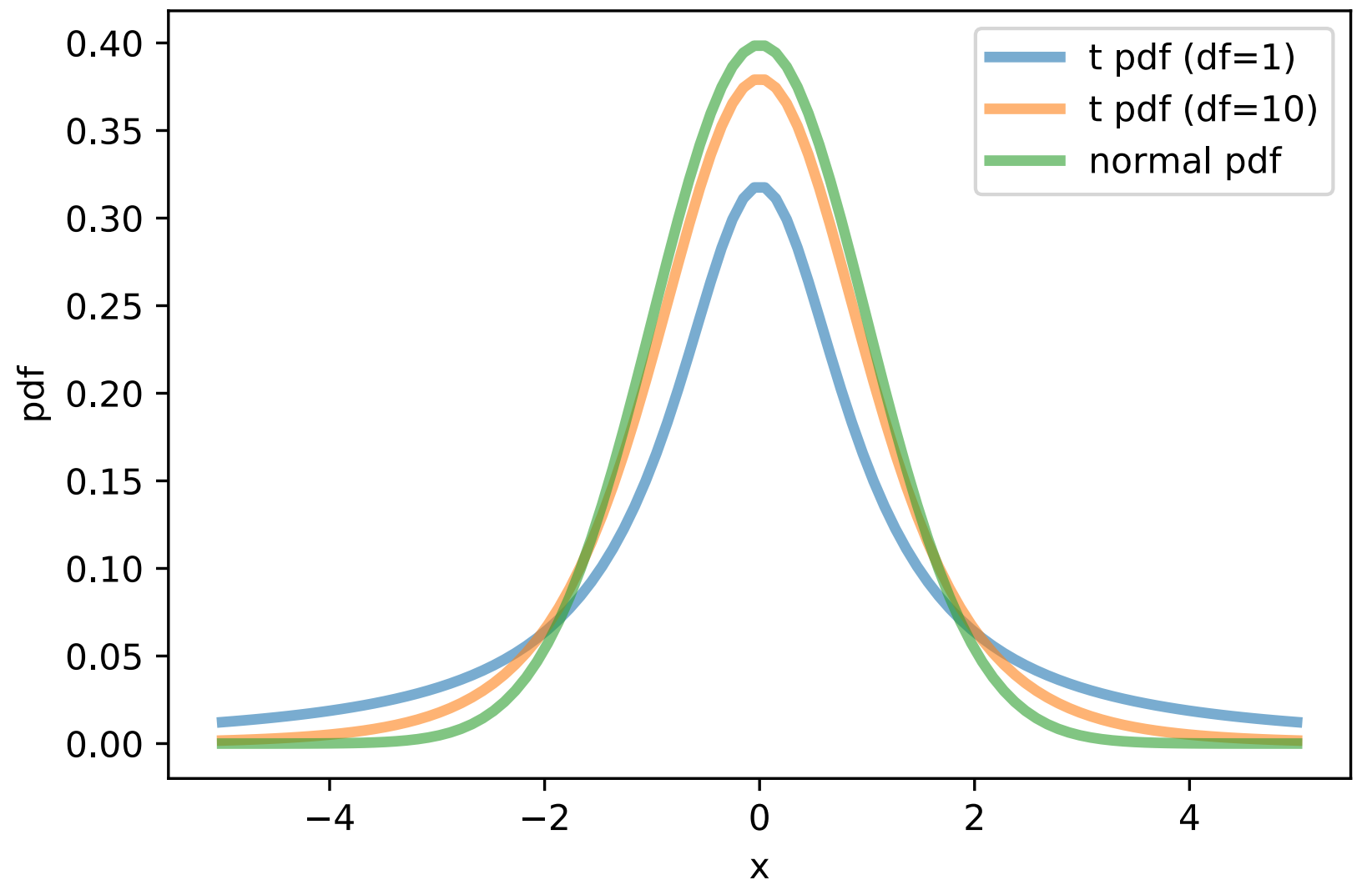
Recall that SNE is trying to minimize the dissimilarity of \(P\) and \(Q\), and \(P\) has a Gaussian distribution. So for a pair of points (\(x_i\) and \(x_j\) in high-dimension, \(y_i\) and \(y_j\) in low-dimension) to reach the same probability, the distance between \(y_i\) and \(y_j\) would be much larger (i.e. much farther apart).
9.1.2.4 Example of t-SNE:
muraro <- readRDS("data/pancreas/muraro.rds")
tmp <- runTSNE(muraro, perplexity = 3)
plotTSNE(tmp, colour_by = "cell_type1")
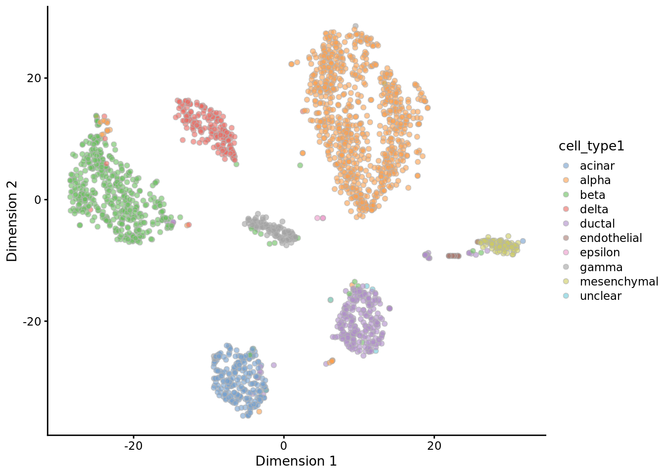
tmp <- runTSNE(muraro, perplexity = 50)
plotTSNE(tmp, colour_by = "cell_type1")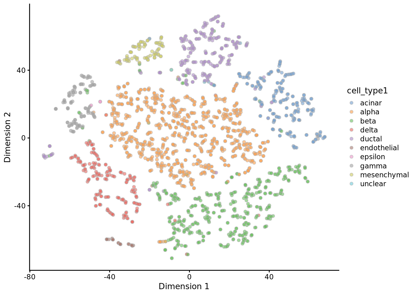
9.1.2.5 Limits of t-SNE:
- Not a convex problem, i.e. the cost function has multiple local minima.
- Non-deterministic.
- Require specification of very important parameters, e.g. perplexity.
- Coordinates after embedding have no meaning.
Therefore can merely be used for visualization.
(See here for more pitfalls of using t-SNE.)
9.1.3 Manifold methods
9.1.3.1 UMAP: Uniform Manifold Approximation and Projection (McInnes, Healy, and Melville 2018)
9.1.3.1.1 Advantages of UMAP over t-SNE:
- faster
- deterministic
- better at preserving clusters
9.1.3.1.2 High level description
- Construct a topological presentation of the high-dimensional data (in this case a weighted \(k\)-NN graph)
- Given a low-dimensional data, construct a graph in the similar way
- Minimize the dissimilarity between the twp graphs.
(Look for the low-dimensional data whose graph is the closest to that of the high-dimensional data)
9.1.3.1.3 Some details
- How the weighted graph is built?
Obtain dissimilarity from the input distance:
For each data point \(x_i\), find its \(k\) nearest neighbours: \(x_{i_1}, \dots, x_{i_k}\).
Let \(d(x_i, x_{i_j})\) be the input or original distance between \(x_i\) and \(x_{i_j}\), and \(\rho_i = \min[d(x_i, x_{i_j}); 1 \leq j \leq k]\) be the distance between \(x_i\) and its nearest neighbour.
Then the dissimilarity between \(x_i\) and \(x_{i_j}\) is measured simply by subtracting the original distance by \(\rho_i\): \(\tilde{d}(x_i, x_{i_j}) = d(x_i, x_{i_j}) - \rho_i\).
Tranform dissimilarity to similarity:
\(s(x_i, x_{i_j}) = \exp[-\tilde{d}(x_i, x_{i_j})] - c_i\), where \(c_i\) is a scale factor to ensure \(\sum_{j = 1}^k s(x_i, x_{i_j})\) is a constant for all \(i\).
Similarity itself can serve as edge weights, but this similarity is not symmetrical, i.e. \(s(x_i, x_{i_j}) \neq s(x_{i_j}, x_i)\). To be able to project this onto an undirected graph, we need to solve the disagreement between \(s(x_i, x_{i_j})\) and \(s(x_{i_j}, x_i)\).Obtain weights:
\(w(x_i, x_{i_j}) = s(x_i, x_{i_j}) + s(x_{i_j}, x_i) - s(x_i, x_{i_j}) * s(x_{i_j}, x_i)\)
(Interpretation: \(P(A \cup B ) = P(A) + P(B) - P(A)P(B)\) if \(A\) and \(B\) are independent)
- How the dissimilarity between graphs are measured? Cross entropy
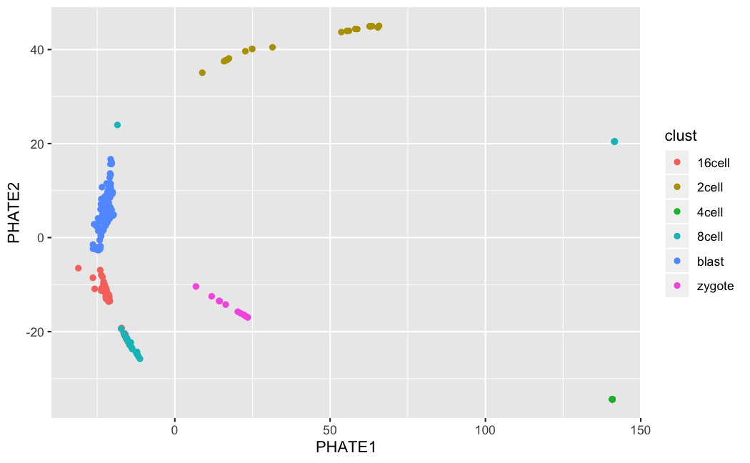
9.1.3.2 PHATE (Moon et al. 2017)
9.1.3.2.1 Sketch of algorithm
The simpliest description of PHATE:
Step1. Create a dissimilarity matrix of the original data
Step2. Feed the dissimilarity matrix to nonmetric MDS
(MDS: Multi-Dimension Scaling is a classical dimensionality reduction approach, that takes an input of distance matrix, and aims at preserving pairwise distances in the low dimensional space. When the input distance matrix is Euclidean distance, MDS produces the same result as PCA. Nonmetric MDS generalize the input as a dissimilarity matrix, rather than just distance.)- Details of step1 in PHATE
Step1-1. Markov transition matrix
- What is similar with SNE:
Recall that in the original SNE algorithm, there is a similarity matrix with entry \(p_{i|j}\) that is interpreted as the probability that point \(x_i\) chooses \(x_j\) as its neighbour: \(p_{j|i} \propto \exp(-\Vert x_i - x_j \Vert^2/2\delta^2)\).
PHATE is doing the same, except that we can interpret it differently:
i. We can think \(p_{j|i}\) as a Gaussian kernel, where \(\epsilon \triangleq 2\delta^2\) is the bandwidth: \(p_{j|i} \triangleq K_\epsilon(x_i, x_j )\). Similar to SNE, PHATE also define \(\epsilon\) as the \(k\)-NN distance of each data point, so that it is smaller in dense area and larger in sparse area. The \(k\) is a user-specified tuning parameter, similar to perplexity in SNE.
ii. We can think of the similarity matrix as a transition matrix, where \(p_{j|i}\) represents the probability of jumping from state \(i\) to state \(j\) in a single step.
- What is different:
i. PHATE generalize \(K_\epsilon(x_i, x_j)\) to \(\exp \left(- \Vert x_i - x_j \Vert^\alpha /\epsilon(x_i)^\alpha\right)\), where the original Gaussian kernel is the special case when \(\alpha = 2\).
The motivation is that if the data is very sparse in some regions, then the bandwith \(\epsilon\) with be very large and the kernel will become flat and lose the local information. By letting \(\alpha > 2\), we prevent this to happen, although \(\alpha\) needs to be provided by the user.
ii. Note that the kernels are not symmetrical now, that is \(K_\epsilon(x_i, x_j) \neq K_\epsilon(x_j, x_i)\). So we make it symmetrical by taking an average of the two.
Step1-2. Smoothing
- \(P\) is the transition matrix where \(p_{i, j}\) represents the probability of jumping from state \(i\) to state \(j\) in a single step.
- Denote \(\delta_x\) as a row vector of length \(n\) (the number of data points), where only the entry corresponding to \(x\) is 1 and zero everywhere else.
Then \(p_x = \delta_x P\) is the probability distribution of the data points starting from \(x\) after one step,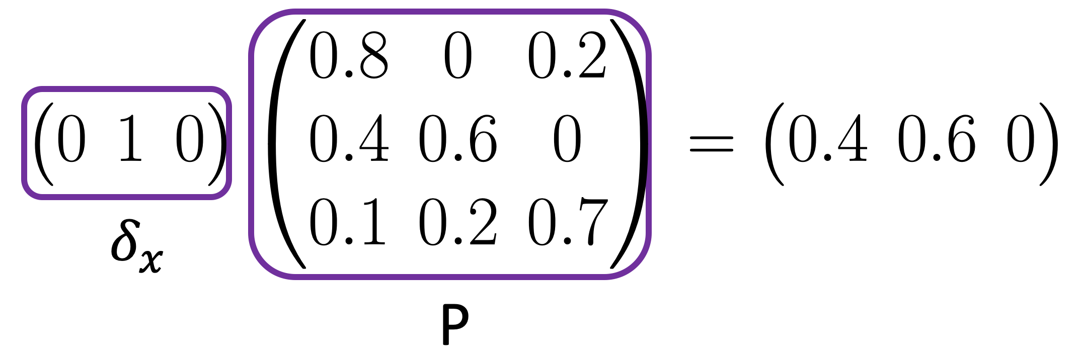
and \(p_x^t = \delta_x P^t\) is the probability distribution of the data points after \(t\) steps.
In general, the more steps we take, the more data points will have positive probabilities.
One way to think about this, is the larger \(t\) is, the more global information and the less local information is encoded.
In the extreme case, if we take infinity steps, \(p_x^\infty\) will be the same for all \(x\)’s, i.e. the probability distribution is going to be the same regardless of where we start, in this case, the local information is completely lost.
An appropriately chosen \(t\) is crucial for the balance between local and global information in the embedding. (See the original paper for details of choosing \(t\))
Step1-3. Distance measurement
Instead of measuring directly the Eudlicean distance between data points, say \(x_i\) and \(x_j\), PHATE measures the distance between probability distributions \(p_{x_i}^t\) and \(p_{x_j}^t\):
\(D^t(x_i, x_j) = \Vert \log(p_{x_i}^t) - \log(p_{x_j}^t) \Vert^2\)
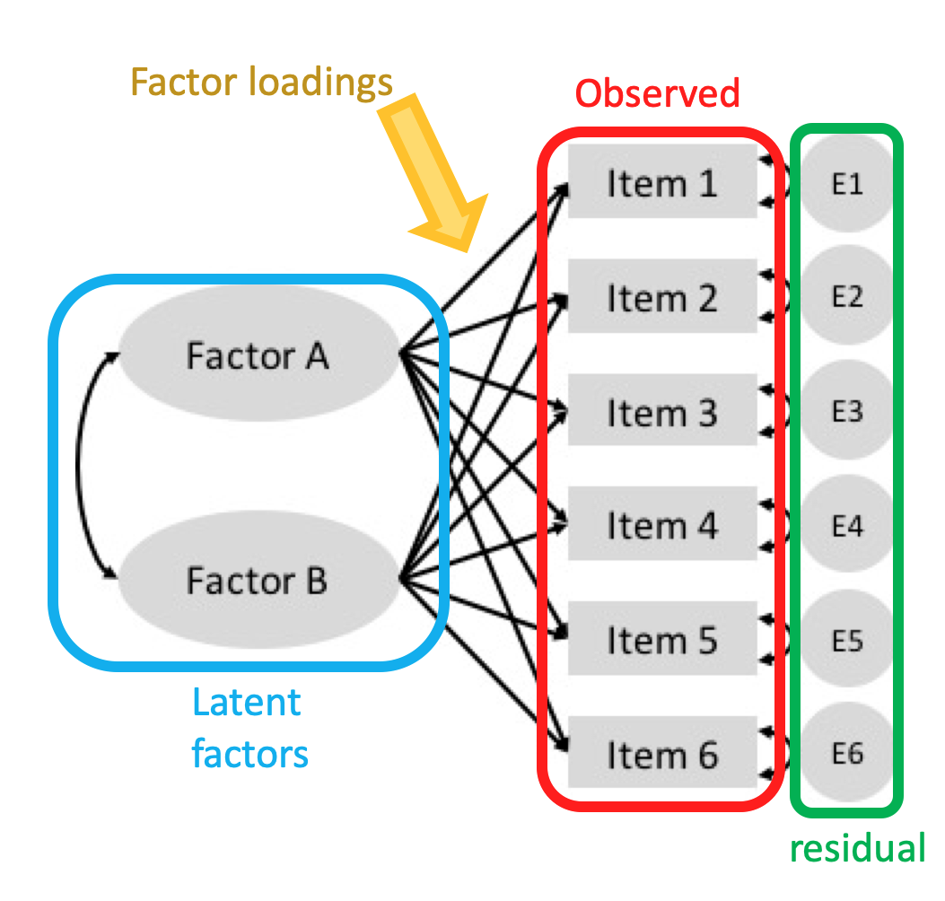
9.2 Matrix factorization and factor analysis
The key concept of factor analysis: The original, observed variables are correlated because they are all associated with some unobservable variables, the latent factors.
It looks similar to PCA, but instead of dimensionality reduction, factor analysis focuses on studying the latent factors.
The variance of an observed variable can be splitted into two parts:
- Common variance: the part of variance that is explained by latent factors;
- Unique variance: the part that is specific to only one variable, usually considered as an error component or residual.
The factor loadings or weights indicate how much each latent factor is affecting the observed features.
9.2.1 Slalom: Interpretable latent spaces
Highlight of Slalom: (Buettner et al. 2017)
It incorporates prior information to help the model estimation;
It learns whatever not provided by prior knowledge in the model training process;
It enforces sparsity in the weight matrix.
9.2.1.1 Methodology
Matrix expression of factor analysis:
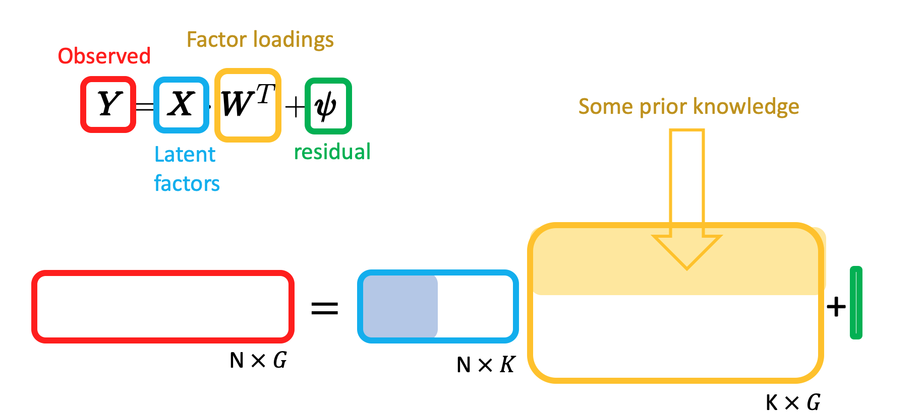
How prior knowledge affects the model:
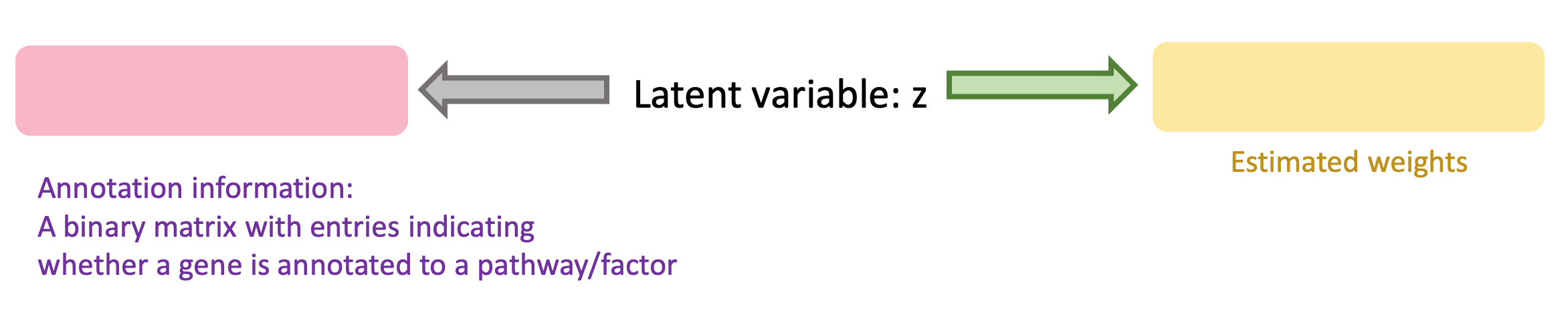
- \(I_{g, k}\): (observed) Indicator of whether a gene \(g\) is annotated to a given pathway or factor \(k\);
- \(z_{g, k}\): (latent) Indicator of whether factor \(k\) has a regulatory effect on gene \(g\);
- \(w_{g, k}\): (estimated) weights.
grey arrow: \[ P(I_{g, k}\vert z_{g, k}) = \begin{cases} \text{Bernoulli}(p_1), \text{if } z_{g, k} = 1\\ \text{Bernoulli}(p_2), \text{if } z_{g, k} = 0\\ \end{cases}\]
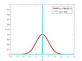
green arrow: \[ P(w_{g, k}\vert z_{g, k}) = \begin{cases} N(w_{g, k}, 1/\alpha), \text{ if } z_{g, k} = 1\\ \delta_0(w_{g, k}), \text{ if } z_{g, k} = 0\\ \end{cases}\]
We only look at the part of the likelihood that is relavant to this part:
\(\prod_{g} \prod_{k}P(I_{g, k}, w_{g, k}, z_{g, k})\),
where \(P(I_{g, k}, w_{g, k}, z_{g, k}) = P(I_{g, k}, w_{g, k}| z_{g, k})P(z_{g,k}) = P( I_{g, k}| z_{g, k})P( w_{g, k}| z_{g, k})P(z_{g,k})\).
Since we do not know anything about \(z_{g,k}\), it is assumed as Bernoulli(1/2).
9.2.1.2 Example
First, get a geneset in a GeneSetCollection object.
gmtfile <- system.file("extdata", "reactome_subset.gmt", package = "slalom")
genesets <- GSEABase::getGmt(gmtfile)
Then we create an Rcpp_SlalomModel object containing the input data and genesets (and subsequent results) for the model.
## 29 annotated factors retained;  1 annotated factors dropped.
## 1072  genes retained for analysis.
Initialize the model:
Fit/train the model:
## pre-training model for faster convergence
## iteration 0
## Model not converged after 50 iterations.
## iteration 0
## Model not converged after 50 iterations.
## iteration 0
## Switched off factor 29
## Switched off factor 20
## Switched off factor 32
## Switched off factor 28
## Switched off factor 13
## Switched off factor 27
## Switched off factor 10
## iteration 100
## Switched off factor 22
## iteration 200
## iteration 300
## iteration 400
## iteration 500
## iteration 600
## iteration 700
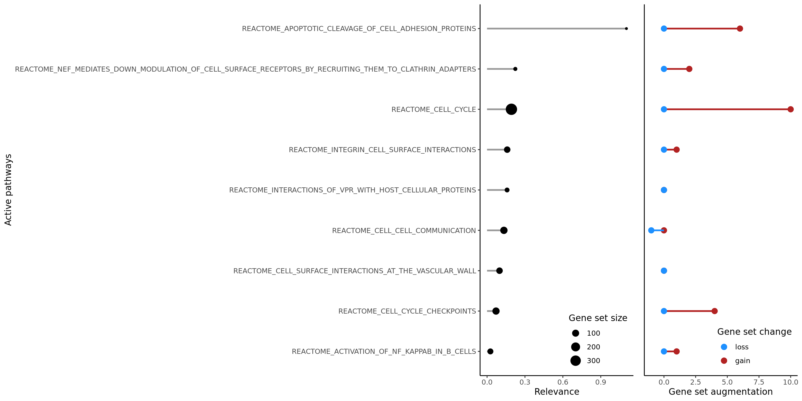
## Model converged after 701 iterations.View results:
The plotRelevance function displays the most relevant terms (factors/pathways) ranked by relevance, showing gene set size and the number of genes gained/lost as active in the pathway as learnt by the model.
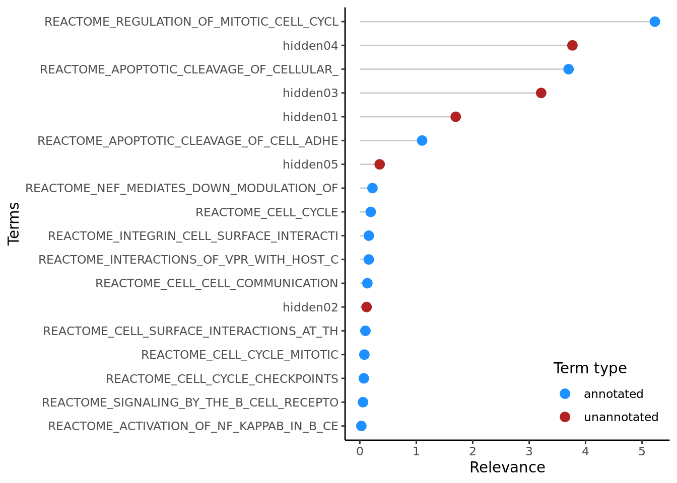
## NULLThe plotTerms function shows the relevance of all terms in the model, enabling the identification of the most important pathways in the context of all that were included in the model.
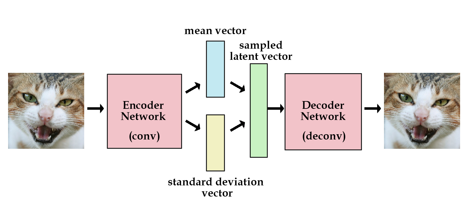
9.3 Autoencoders
(Kingma and Welling 2013)
9.3.1 Background and some notations
- Data: \(X\)
Latent variables: \(Z\)
Something that is not directly observable but is assumed to have an impact on the observed variables.Goal: We believe \(X\) can be generated from \(Z\) (with some trasformation), and want to sample more data from \(Z\) that resembles \(X\). So we want the to find the parameters \(\theta\) such that the probability to generate \(X\) from the distribution of \(Z\): \(P(X) = \int P(X|z; \theta) P(z) dz\) is maximized.
- How do we define \(Z\)?
- The simplest idea: \(Z \sim N(0, 1)\).
It is not impossible, because “any distribution in d dimensions can be generated by taking a set of d variables that are normally distributed and mapping them through a sufficiently complicated function.”
-A better idea: For most of \(z\), \(P(X|z; \theta)\) will be close to zero, meaning it contribute almost nothing to the estimate of \(P(X)\). Thus, we want to sample only those values of \(Z\) that are likely to produce \(X\). Denote this distribution of \(Z\) as \(Q(Z|X)\) (it is infered and therefore depend on \(X\)).
Advantage: There will be a lot less possible values of \(Z\) under \(Q\) compared to random sampling, therefore, it will be easier to compute \(E_{Z \sim Q} P(X|Z)\).
- The simplest idea: \(Z \sim N(0, 1)\).
It is not impossible, because “any distribution in d dimensions can be generated by taking a set of d variables that are normally distributed and mapping them through a sufficiently complicated function.”
9.3.2 Objective
\[ \log P(X) - KL[Q(Z|X)\Vert P(Z|X)] = E_{Z\sim Q}[\log P(X|Z)] - KL[Q(Z|X)\Vert P(Z)]\] We can get this equation by starting from the definition of Kullback-Leibler divergence, combined with the Bayesian formula and a little algebra. (Not showing details here)
- LHS: what we want to maximize:
Generation loss: how likely the generated samples resembles \(X\) -
an error term which measures how much information is lost when using \(Q\) to represent \(P\),
it becomes small if \(Q\) is high-capacity.
(A loose explanation of model capacity: Roughly speaking, the capacity of a model describes how complex a relationship it can model. You could expect a model with higher capacity to be able to model more relationships between more variables than a model with a lower capacity.)
- RHS: what we can maximize through stochastic gradient descent.
References
Buettner, Florian, Naruemon Pratanwanich, Davis J McCarthy, John C Marioni, and Oliver Stegle. 2017. “F-scLVM: Scalable and Versatile Factor Analysis for Single-Cell Rna-Seq.” Genome Biology 18 (1). BioMed Central: 212.
Collins, Michael, Sanjoy Dasgupta, and Robert E Schapire. 2002. “A Generalization of Principal Components Analysis to the Exponential Family.” In Advances in Neural Information Processing Systems, 617–24.
Hinton, Geoffrey E, and Sam T Roweis. 2003. “Stochastic Neighbor Embedding.” In Advances in Neural Information Processing Systems, 857–64.
Kingma, Diederik P, and Max Welling. 2013. “Auto-Encoding Variational Bayes.” arXiv Preprint arXiv:1312.6114.
Maaten, Laurens van der, and Geoffrey Hinton. 2008. “Visualizing Data Using T-Sne.” Journal of Machine Learning Research 9 (Nov): 2579–2605.
McInnes, Leland, John Healy, and James Melville. 2018. “Umap: Uniform Manifold Approximation and Projection for Dimension Reduction.” arXiv Preprint arXiv:1802.03426.
Moon, Kevin R, David van Dijk, Zheng Wang, William Chen, Matthew J Hirn, Ronald R Coifman, Natalia B Ivanova, Guy Wolf, and Smita Krishnaswamy. 2017. “PHATE: A Dimensionality Reduction Method for Visualizing Trajectory Structures in High-Dimensional Biological Data.” bioRxiv. Cold Spring Harbor Laboratory, 120378.
Townes, F William, Stephanie C Hicks, Martin J Aryee, and Rafael A Irizarry. 2019. “Feature Selection and Dimension Reduction for Single Cell Rna-Seq Based on a Multinomial Model.” bioRxiv. Cold Spring Harbor Laboratory, 574574.