6 Quality control and data visualisation
The principle of garbage in, garbage out is at least as strong in single-cell genomics as it is elsewere in science. Effective quality control (QC) is crucial to high-quality scRNA-seq data analysis. We discuss principles and strategies for QC in this chapter, along with some discussion and demonstration of data visualisation approaches.
6.1 Expression QC overview (UMI)
6.1.1 Introduction
Once gene expression has been quantified it is summarized as an expression matrix where each row corresponds to a gene (or transcript) and each column corresponds to a single cell. This matrix should be examined to remove poor quality cells which were not detected in either read QC or mapping QC steps. Failure to remove low quality cells at this stage may add technical noise which has the potential to obscure the biological signals of interest in the downstream analysis.
Since there is currently no standard method for performing scRNASeq the expected values for the various QC measures that will be presented here can vary substantially from experiment to experiment. Thus, to perform QC we will be looking for cells which are outliers with respect to the rest of the dataset rather than comparing to independent quality standards. Consequently, care should be taken when comparing quality metrics across datasets collected using different protocols.
6.1.2 Tung dataset
To illustrate cell QC, we consider a
dataset of induced
pluripotent stem cells generated from three different individuals (Tung et al. 2017)
in Yoav Gilad’s lab at the University of
Chicago. The experiments were carried out on the Fluidigm C1 platform and to
facilitate the quantification both unique molecular identifiers (UMIs) and ERCC
spike-ins were used. The data files are located in the tung folder in your
working directory. These files are the copies of the original files made on the
15/03/16. We will use these copies for reproducibility purposes.
Load the data and annotations:
molecules <- read.table("data/tung/molecules.txt", sep = "\t")
anno <- read.table("data/tung/annotation.txt", sep = "\t", header = TRUE)
Inspect a small portion of the expression matrix
##                 NA19098.r1.A01 NA19098.r1.A02 NA19098.r1.A03
## ENSG00000237683              0              0              0
## ENSG00000187634              0              0              0
## ENSG00000188976              3              6              1
## ENSG00000187961              0              0              0
## ENSG00000187583              0              0              0
## ENSG00000187642 0 0 0## individual replicate well batch sample_id
## 1 NA19098 r1 A01 NA19098.r1 NA19098.r1.A01
## 2 NA19098 r1 A02 NA19098.r1 NA19098.r1.A02
## 3 NA19098 r1 A03 NA19098.r1 NA19098.r1.A03
## 4 NA19098 r1 A04 NA19098.r1 NA19098.r1.A04
## 5 NA19098 r1 A05 NA19098.r1 NA19098.r1.A05
## 6 NA19098 r1 A06 NA19098.r1 NA19098.r1.A06The data consists of 3 individuals and r length(unique(anno$replicate)) replicates and therefore has r length(unique(anno$batch)) batches in total.
We standardize the analysis by using both SingleCellExperiment (SCE) and
scater packages. First, create the SCE object:
Remove genes that are not expressed in any cell:
Define control features (genes) - ERCC spike-ins and mitochondrial genes (provided by the authors):
isSpike(umi, "ERCC") <- grepl("^ERCC-", rownames(umi))
isSpike(umi, "MT") <- rownames(umi) %in%
    c("ENSG00000198899", "ENSG00000198727", "ENSG00000198888",
    "ENSG00000198886", "ENSG00000212907", "ENSG00000198786",
    "ENSG00000198695", "ENSG00000198712", "ENSG00000198804",
    "ENSG00000198763", "ENSG00000228253", "ENSG00000198938",
    "ENSG00000198840")
Calculate the quality metrics:
umi <- calculateQCMetrics(
    umi,
    feature_controls = list(
        ERCC = isSpike(umi, "ERCC"),
        MT = isSpike(umi, "MT")
    )
)
## Warning in calculateQCMetrics(umi, feature_controls = list(ERCC =
## isSpike(umi, : spike-in set 'ERCC' overwritten by feature_controls set of
## the same name6.2 Cell QC
6.2.1 Library size
Next we consider the total number of RNA molecules detected per sample (if we were using read counts rather than UMI counts this would be the total number of reads). Wells with few reads/molecules are likely to have been broken or failed to capture a cell, and should thus be removed.
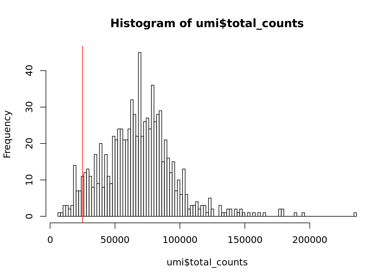
Figure 6.1: Histogram of library sizes for all cells
Exercise 1
How many cells does our filter remove?
What distribution do you expect that the total number of molecules for each cell should follow?
Our answer
## filter_by_total_counts
## FALSE  TRUE
##    46   818
6.2.2 Detected genes
In addition to ensuring sufficient sequencing depth for each sample, we also want to make sure that the reads are distributed across the transcriptome. Thus, we count the total number of unique genes detected in each sample.
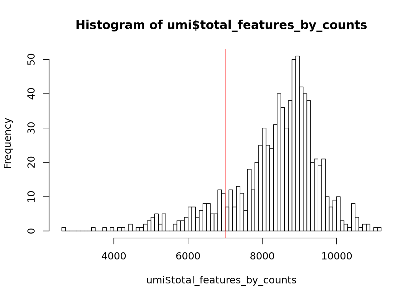
Figure 6.2: Histogram of the number of detected genes in all cells
From the plot we conclude that most cells have between 7,000-10,000 detected genes, which is normal for high-depth scRNA-seq. However, this varies by experimental protocol and sequencing depth. For example, droplet-based methods or samples with lower sequencing-depth typically detect fewer genes per cell. The most notable feature in the above plot is the “heavy tail” on the left hand side of the distribution. If detection rates were equal across the cells then the distribution should be approximately normal. Thus we remove those cells in the tail of the distribution (fewer than 7,000 detected genes).
Exercise 2
How many cells does our filter remove?
Our answer
## filter_by_expr_features
## FALSE  TRUE
##   116   748
6.2.3 ERCCs and MTs
Another measure of cell quality is the ratio between ERCC spike-in RNAs and endogenous RNAs. This ratio can be used to estimate the total amount of RNA in the captured cells. Cells with a high level of spike-in RNAs had low starting amounts of RNA, likely due to the cell being dead or stressed which may result in the RNA being degraded.
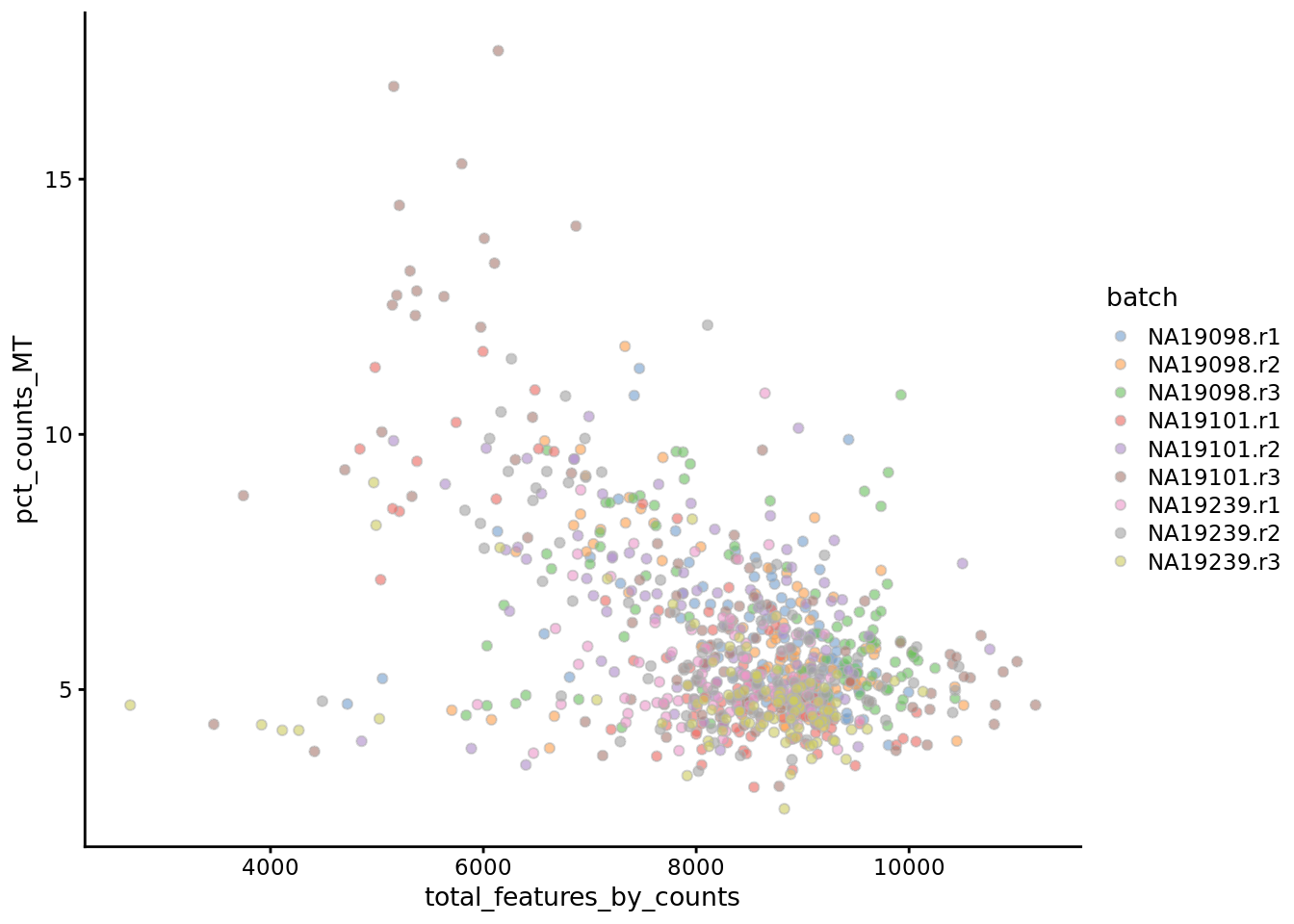
Figure 6.3: Percentage of counts in MT genes
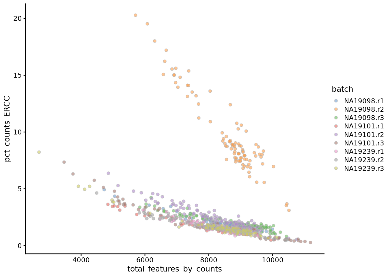
Figure 6.4: Percentage of counts in ERCCs
The above analysis shows that majority of the cells from NA19098.r2 batch have a very high ERCC/Endo ratio. Indeed, it has been shown by the authors that this batch contains cells of smaller size.
Exercise 3
Create filters for removing batch NA19098.r2 and cells with high expression of mitochondrial genes (>10% of total counts in a cell).
Our answer
## filter_by_ERCC
## FALSE  TRUE
##    96   768
## filter_by_MT
## FALSE TRUE
## 31 833Exercise 4
What would you expect to see in the ERCC vs counts plot if you were examining a dataset containing cells of different sizes (eg. normal & senescent cells)?
Answer
You would expect to see a group corresponding to the smaller cells (normal) with a higher fraction of ERCC reads than a separate group corresponding to the larger cells (senescent).
6.2.4 Cell filtering
6.2.4.1 Manual
Now we can define a cell filter based on our previous analysis:
umi$use <- (
    # sufficient features (genes)
    filter_by_expr_features &
    # sufficient molecules counted
    filter_by_total_counts &
    # sufficient endogenous RNA
    filter_by_ERCC &
    # remove cells with unusual number of reads in MT genes
    filter_by_MT
)##
## FALSE TRUE
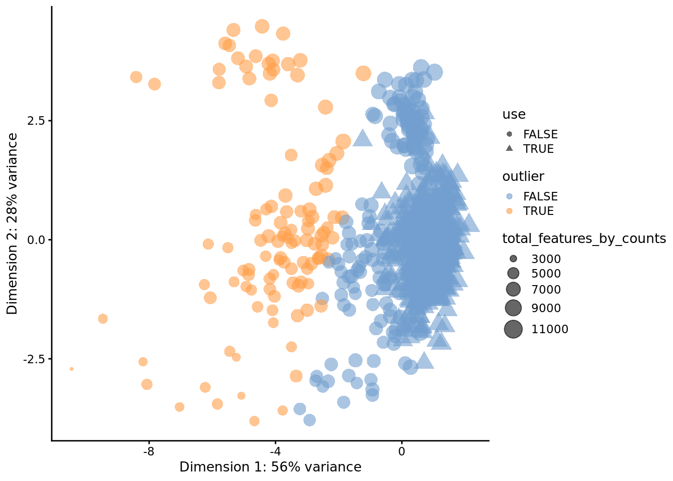
## 207 6576.2.4.2 Automatic
Another option available in scater is to conduct PCA on a set of QC metrics
and then use automatic outlier detection to identify potentially problematic
cells.
By default, the following metrics are used for PCA-based outlier detection:
- pct_counts_top_100_features
- total_features
- pct_counts_feature_controls
- n_detected_feature_controls
- log10_counts_endogenous_features
- log10_counts_feature_controls
scater first creates a matrix where the rows represent cells and the columns
represent the different QC metrics. Then, outlier cells can also be identified
by using the mvoutlier package on the QC metrics for all cells. This will
identify cells that have substantially different QC metrics from the others,
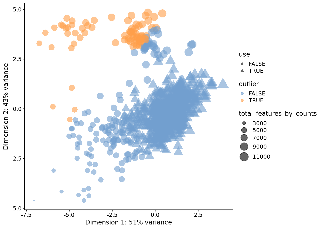
possibly corresponding to low-quality cells. We can visualize any outliers using
a principal components plot as shown below:
## [1] "PCA_coldata"Column subsetting can then be performed based on the $outlier slot, which
indicates whether or not each cell has been designated as an outlier. Automatic
outlier detection can be informative, but a close inspection of QC metrics and
tailored filtering for the specifics of the dataset at hand is strongly
recommended.
##
## FALSE  TRUE
##   791    73
Then, we can use a PCA plot to see a 2D representation of the cells ordered by their quality metrics.
plotReducedDim(
    umi,
    use_dimred = "PCA_coldata",
    size_by = "total_features_by_counts",
    shape_by = "use",
    colour_by = "outlier"
)
6.2.5 Compare filterings
Exercise 5
Compare the default, automatic and manual cell filters. Plot a Venn diagram of the outlier cells from these filterings.
Hint: Use vennCounts and vennDiagram functions from the limma package to make a Venn diagram.
Answer
library(limma)
auto <- colnames(umi)[umi$outlier]
man <- colnames(umi)[!umi$use]
venn.diag <- vennCounts(
    cbind(colnames(umi) %in% auto,
    colnames(umi) %in% man)
)
vennDiagram(
    venn.diag,
    names = c("Automatic", "Manual"),
    circle.col = c("blue", "green")
)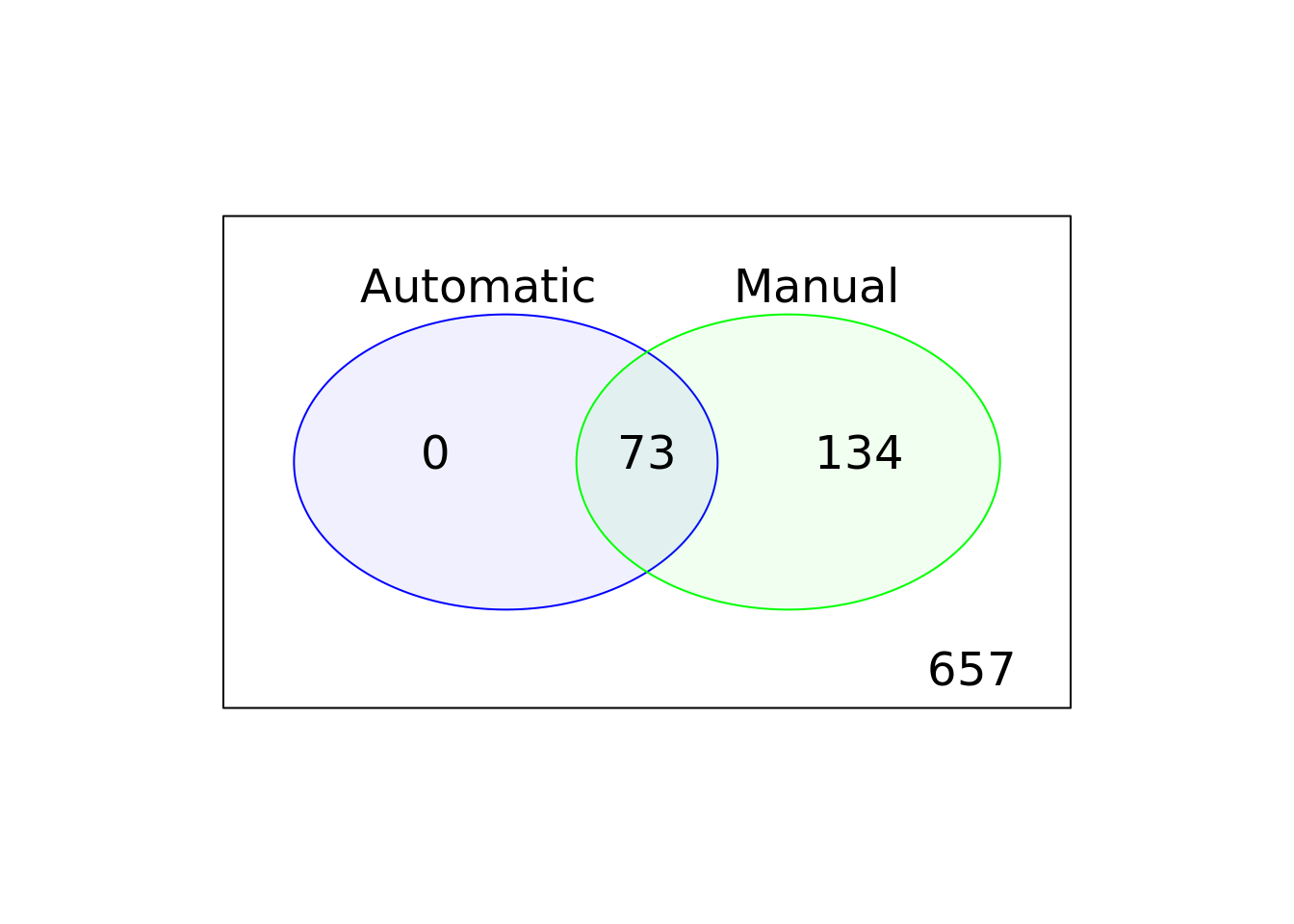
Figure 6.5: Comparison of the default, automatic and manual cell filters
6.3 Doublet detection
For droplet-based datasets, there is chance that multiple cells are enclosed in one droplet resulting one cell barcode actually containing read information from multiple cells. One way to find doublets/multiplets in the data is to see if there are cells co-expressing markers of distinct cell types. There are also computational tools available for detecting potential doublets in the cells. A lot of these tools rely on artificial doublets formed from the datasets by randomly joining the expression profiles of two cells. Then the cells are tested against the artificial doublet profiles.
We demonstrate the usage of two of these doublet detection tools.
6.3.1 scds
scds(Bais and Kostka 2019) has two detection methods:
- co-expression based;
- binary-classification based.
In co-expression based approach, the gene-pairs’ co-expression probablities are estimated based on a binomial model and gene pairs that do not co-expression often get higher scores when they co-expression in some cells. The cells’ doublet scores are derived based on the co-expression of pairs of genes. In the binary classification based approach, artificial doublet clusters are generated and cells are difficult to separate from the artificial doublets get higher doublet scores.
library(scds)
#- Annotate doublet using co-expression based doublet scoring:
umi = cxds(umi)

#- Annotate doublet using binary classification based doublet scoring:
umi = bcds(umi)
## [1] train-error:0.066402+0.005931 test-error:0.103638+0.025177
## Multiple eval metrics are present. Will use test_error for early stopping.
## Will train until test_error hasn't improved in 2 rounds.
##
## [2] train-error:0.049912+0.002718 test-error:0.085687+0.015561
## [3] train-error:0.036747+0.002381 test-error:0.079870+0.015979
## [4] train-error:0.029948+0.002910 test-error:0.071214+0.015731
## [5] train-error:0.026042+0.003332 test-error:0.072934+0.012966
## [6] train-error:0.022424+0.002773 test-error:0.064263+0.011326
## [7] train-error:0.019385+0.003075 test-error:0.058461+0.012930
## [8] train-error:0.018084+0.001510 test-error:0.056722+0.009848
## [9] train-error:0.016203+0.002440 test-error:0.052094+0.012606
## [10] train-error:0.013310+0.003702 test-error:0.049775+0.013542
## [11] train-error:0.011574+0.002856 test-error:0.046891+0.012536
## [12] train-error:0.010705+0.001959 test-error:0.046302+0.011468
## [13] train-error:0.009693+0.001081 test-error:0.043413+0.012598
## [14] train-error:0.008826+0.000545 test-error:0.042254+0.011269
## [15] train-error:0.007813+0.000709 test-error:0.040515+0.011465
## [16] train-error:0.006655+0.000705 test-error:0.042249+0.011692
## [17] train-error:0.005498+0.000584 test-error:0.042254+0.012804
## Stopping. Best iteration:
## [15] train-error:0.007813+0.000709 test-error:0.040515+0.011465
##
## [1] train-error:0.068866
## Will train until train_error hasn't improved in 2 rounds.
##
## [2] train-error:0.038194
## [3] train-error:0.034144
## [4] train-error:0.026620
## [5] train-error:0.024884
## [6] train-error:0.020255
## [7] train-error:0.020255
## [8] train-error:0.019097
## [9] train-error:0.016782
## [10] train-error:0.013310#- Combine both annotations into a hybrid annotation
umi = cxds_bcds_hybrid(umi)
#- Doublet scores are now available via colData:
CD = colData(umi)
head(cbind(CD$cxds_score,CD$bcds_score, CD$hybrid_score))## [,1] [,2] [,3]
## NA19098.r1.A01 4131.405 0.012810320 0.2455279
## NA19098.r1.A02 4564.089 0.004930826 0.2628488
## NA19098.r1.A03 2827.904 0.020504847 0.1769445
## NA19098.r1.A04 4708.213 0.009793874 0.2762736
## NA19098.r1.A05 6134.590 0.006487557 0.3565501
## NA19098.r1.A06 5810.730 0.008279418 0.3393878
The scds paper features
excellent descriptions and evaluations of other currently-available doublet
detection methods.
6.3.2 DoubletDetection
DoubletDetection is a python module that runs on raw UMI counts data. It generates artificial doublets and then perform cell clustering using the augmented dataset. Cells cluster closely to the artificial doublets across multiple iterations are predicted to be doublets.
We provided the python scripts for running DoubletDetection on Tung datasets at ./mig_2019_scrnaseq-workshop/course_files/utils/run_doubletDetection.py
python run_doubletDetection.py
Here is the prediction results by DoubletDetection:
## Loading required package: UpSetR## [1] 864 1## [1] 864 5umi$dbd_dbl <- factor(pred_tung$V1)
qc_label <- read.delim(file = "data/qc_ipsc.txt")
head(qc_label)## individual replicate well cell_number concentration tra1.60
## 1 NA19098 r1 A01 1 1.734785 1
## 2 NA19098 r1 A02 1 1.723038 1
## 3 NA19098 r1 A03 1 1.512786 1
## 4 NA19098 r1 A04 1 1.347492 1
## 5 NA19098 r1 A05 1 2.313047 1
## 6 NA19098 r1 A06 1 2.056803 1qc_label$sample_id <- paste0(qc_label$individual,".",qc_label$replicate,".",qc_label$well)
rownames(qc_label) <- qc_label$sample_id
umi$cell_number <- as.character(qc_label[umi$sample_id,"cell_number"])
umi$cell_number[qc_label$cell_number==0] <- "no_cell"
umi$cell_number[qc_label$cell_number == 1] <- "single_cell"
umi$cell_number[qc_label$cell_number>1] <- "multi_cell"
multiplot(plotColData(
umi,
x = "total_features_by_counts",
y = "pct_counts_ERCC",
colour = "hybrid_score"
),
plotColData(
umi,
x = "total_features_by_counts",
y = "pct_counts_ERCC",
colour = "dbd_dbl"
), plotColData(
umi,
x = "total_features_by_counts",
y = "pct_counts_ERCC",
colour = "cell_number"
),cols =2)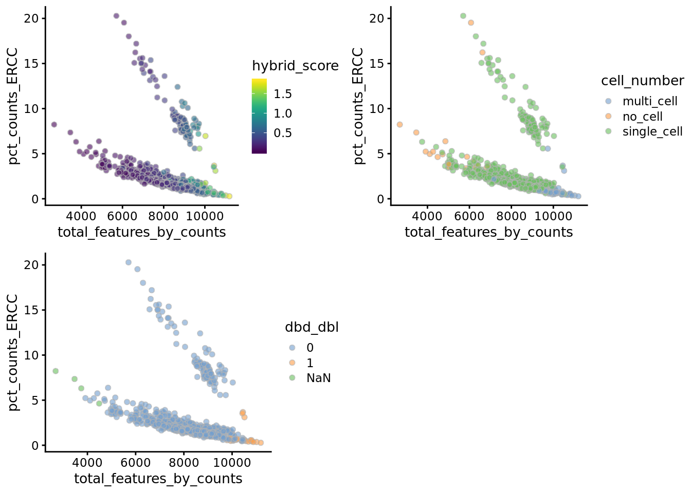
doublets <- unique(umi$sample_id[umi$dbd_dbl =="1"],
                   umi$sample_id[umi$hybrid_score > 0.8])


pl_list <- UpSetR::fromList(list(pred = doublets,qc_label = qc_label$sample_id[qc_label$cell_number >1]))
UpSetR::upset(pl_list,sets = c("pred","qc_label"))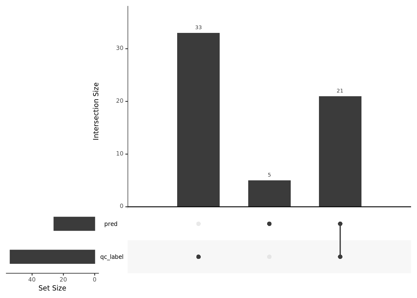
6.3.2.1 Other tools available:
- DoubletFinder
- DoubletCells as part of SimpleSingleCell
- Scrublet
6.4 Gene QC
6.4.1 Gene expression
In addition to removing cells with poor quality, it is usually a good idea to exclude genes where we suspect that technical artefacts may have skewed the results. Moreover, inspection of the gene expression profiles may provide insights about how the experimental procedures could be improved.
It is often instructive to consider the number of reads consumed by the top 50 expressed genes.
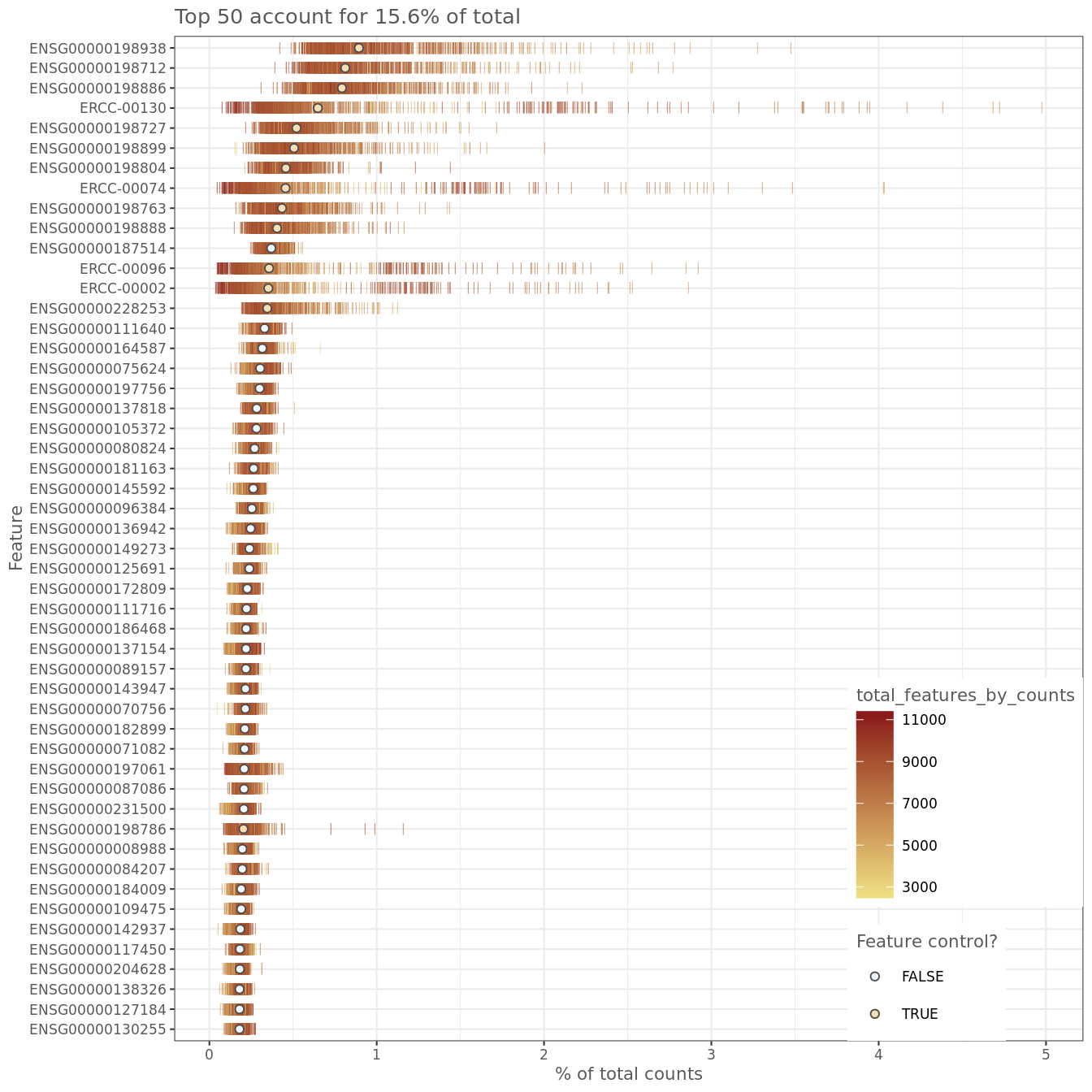
Figure 6.6: Number of total counts consumed by the top 50 expressed genes
The distributions are relatively flat indicating (but not guaranteeing!) good coverage of the full transcriptome of these cells. However, there are several spike-ins in the top 15 genes which suggests a greater dilution of the spike-ins may be preferrable if the experiment is to be repeated.
6.4.2 Gene filtering
It is typically a good idea to remove genes whose expression level is considered
“undetectable”. We define a gene as detectable if at least two cells contain
more than 1 transcript from the gene. If we were considering read counts rather
than UMI counts a reasonable threshold is to require at least five reads in at
least two cells. However, in both cases the threshold strongly depends on the
sequencing depth. It is important to keep in mind that genes must be filtered
after cell filtering since some genes may only be detected in poor quality cells
(note colData(umi)$use filter applied to the umi dataset).
keep_feature <- nexprs(
  umi[,colData(umi)$use],
  byrow = TRUE,
  detection_limit = 1
) >= 2
rowData(umi)$use <- keep_feature## keep_feature
## FALSE TRUE
## 4660 14066Depending on the cell-type, protocol and sequencing depth, other cut-offs may be appropriate.
6.4.3 Save the data
Dimensions of the QCed dataset (do not forget about the gene filter we defined above):
## [1] 14066 657Let’s create an additional slot with log-transformed counts (we will need it in
the next chapters) and remove saved PCA results from the reducedDim slot:
Save the data:
6.4.4 Big Exercise
Perform exactly the same QC analysis with read counts of the same Blischak data.
Use tung/reads.txt file to load the reads. Once you have finished please
compare your results to ours (next chapter).
6.4.5 sessionInfo()
## R version 3.6.0 (2019-04-26)
## Platform: x86_64-pc-linux-gnu (64-bit)
## Running under: Ubuntu 18.04.3 LTS
##
## Matrix products: default
## BLAS:   /usr/lib/x86_64-linux-gnu/blas/libblas.so.3.7.1
## LAPACK: /usr/lib/x86_64-linux-gnu/lapack/liblapack.so.3.7.1
##
## locale:
##  [1] LC_CTYPE=en_AU.UTF-8       LC_NUMERIC=C
##  [3] LC_TIME=en_AU.UTF-8        LC_COLLATE=en_AU.UTF-8
##  [5] LC_MONETARY=en_AU.UTF-8    LC_MESSAGES=en_AU.UTF-8
##  [7] LC_PAPER=en_AU.UTF-8       LC_NAME=C
##  [9] LC_ADDRESS=C               LC_TELEPHONE=C
## [11] LC_MEASUREMENT=en_AU.UTF-8 LC_IDENTIFICATION=C
##
## attached base packages:
## [1] parallel  stats4    stats     graphics  grDevices utils     datasets
## [8] methods   base
##
## other attached packages:
##  [1] UpSetR_1.4.0                scds_1.0.0
##  [3] limma_3.40.6                scater_1.12.2
##  [5] ggplot2_3.2.1               SingleCellExperiment_1.6.0
##  [7] SummarizedExperiment_1.14.1 DelayedArray_0.10.0
##  [9] BiocParallel_1.18.1         matrixStats_0.55.0
## [11] Biobase_2.44.0              GenomicRanges_1.36.1
## [13] GenomeInfoDb_1.20.0         IRanges_2.18.3
## [15] S4Vectors_0.22.1            BiocGenerics_0.30.0
##
## loaded via a namespace (and not attached):
##   [1] ggbeeswarm_0.6.0         colorspace_1.4-1
##   [3] mvoutlier_2.0.9          class_7.3-15
##   [5] modeltools_0.2-22        rio_0.5.16
##   [7] mclust_5.4.5             XVector_0.24.0
##   [9] pls_2.7-1                BiocNeighbors_1.2.0
##  [11] cvTools_0.3.2            flexmix_2.3-15
##  [13] mvtnorm_1.0-11           ranger_0.11.2
##  [15] splines_3.6.0            sROC_0.1-2
##  [17] robustbase_0.93-5        knitr_1.25
##  [19] zeallot_0.1.0            robCompositions_2.1.0
##  [21] kernlab_0.9-27           cluster_2.1.0
##  [23] rrcov_1.4-7              compiler_3.6.0
##  [25] backports_1.1.4          assertthat_0.2.1
##  [27] Matrix_1.2-17            lazyeval_0.2.2
##  [29] BiocSingular_1.0.0       htmltools_0.3.6
##  [31] tools_3.6.0              rsvd_1.0.2
##  [33] gtable_0.3.0             glue_1.3.1
##  [35] GenomeInfoDbData_1.2.1   dplyr_0.8.3
##  [37] Rcpp_1.0.2               carData_3.0-2
##  [39] cellranger_1.1.0         zCompositions_1.3.2-1
##  [41] vctrs_0.2.0              sgeostat_1.0-27
##  [43] fpc_2.2-3                DelayedMatrixStats_1.6.1
##  [45] lmtest_0.9-37            xfun_0.9
##  [47] laeken_0.5.0             stringr_1.4.0
##  [49] openxlsx_4.1.0.1         lifecycle_0.1.0
##  [51] irlba_2.3.3              DEoptimR_1.0-8
##  [53] zlibbioc_1.30.0          MASS_7.3-51.1
##  [55] zoo_1.8-6                scales_1.0.0
##  [57] VIM_4.8.0                hms_0.5.1
##  [59] RColorBrewer_1.1-2       yaml_2.2.0
##  [61] curl_4.2                 NADA_1.6-1
##  [63] gridExtra_2.3            reshape_0.8.8
##  [65] stringi_1.4.3            highr_0.8
##  [67] pcaPP_1.9-73             e1071_1.7-2
##  [69] boot_1.3-20              zip_2.0.4
##  [71] truncnorm_1.0-8          rlang_0.4.0
##  [73] pkgconfig_2.0.3          prabclus_2.3-1
##  [75] bitops_1.0-6             evaluate_0.14
##  [77] lattice_0.20-38          purrr_0.3.2
##  [79] labeling_0.3             cowplot_1.0.0
##  [81] tidyselect_0.2.5         GGally_1.4.0
##  [83] plyr_1.8.4               magrittr_1.5
##  [85] bookdown_0.13            R6_2.4.0
##  [87] pillar_1.4.2             haven_2.1.1
##  [89] foreign_0.8-70           withr_2.1.2
##  [91] survival_2.43-3          abind_1.4-5
##  [93] RCurl_1.95-4.12          sp_1.3-1
##  [95] nnet_7.3-12              tibble_2.1.3
##  [97] crayon_1.3.4             car_3.0-3
##  [99] xgboost_0.90.0.2         rmarkdown_1.15
## [101] viridis_0.5.1            grid_3.6.0
## [103] readxl_1.3.1             data.table_1.12.2
## [105] forcats_0.4.0            diptest_0.75-7
## [107] vcd_1.4-4                digest_0.6.21
## [109] tidyr_1.0.0              munsell_0.5.0
## [111] beeswarm_0.2.3           viridisLite_0.3.0
## [113] vipor_0.4.5
6.5 Exercise: Expression QC (Reads)
reads <- read.table("data/tung/reads.txt", sep = "\t")
anno <- read.table("data/tung/annotation.txt", sep = "\t", header = TRUE)## NA19098.r1.A01 NA19098.r1.A02 NA19098.r1.A03
## ENSG00000237683 0 0 0
## ENSG00000187634 0 0 0
## ENSG00000188976 57 140 1
## ENSG00000187961 0 0 0
## ENSG00000187583 0 0 0
## ENSG00000187642 0 0 0## individual replicate well batch sample_id
## 1 NA19098 r1 A01 NA19098.r1 NA19098.r1.A01
## 2 NA19098 r1 A02 NA19098.r1 NA19098.r1.A02
## 3 NA19098 r1 A03 NA19098.r1 NA19098.r1.A03
## 4 NA19098 r1 A04 NA19098.r1 NA19098.r1.A04
## 5 NA19098 r1 A05 NA19098.r1 NA19098.r1.A05
## 6 NA19098 r1 A06 NA19098.r1 NA19098.r1.A06isSpike(reads, "ERCC") <- grepl("^ERCC-", rownames(reads))
isSpike(reads, "MT") <- rownames(reads) %in%
c("ENSG00000198899", "ENSG00000198727", "ENSG00000198888",
"ENSG00000198886", "ENSG00000212907", "ENSG00000198786",
"ENSG00000198695", "ENSG00000198712", "ENSG00000198804",
"ENSG00000198763", "ENSG00000228253", "ENSG00000198938",
"ENSG00000198840")reads <- calculateQCMetrics(
reads,
feature_controls = list(
ERCC = isSpike(reads, "ERCC"),
MT = isSpike(reads, "MT")
)
)## Warning in calculateQCMetrics(reads, feature_controls = list(ERCC =
## isSpike(reads, : spike-in set 'ERCC' overwritten by feature_controls set of
## the same name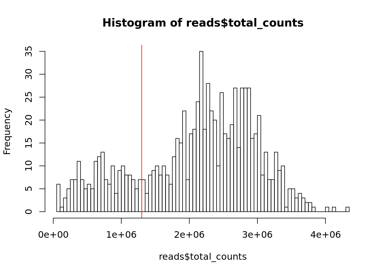
Figure 6.7: Histogram of library sizes for all cells
## filter_by_total_counts
## FALSE  TRUE
##   180   684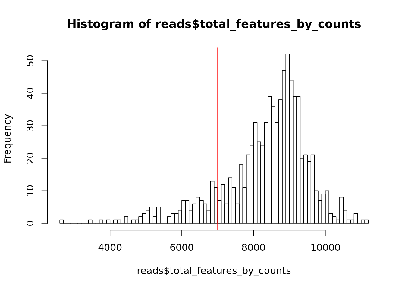
Figure 6.8: Histogram of the number of detected genes in all cells
## filter_by_expr_features
## FALSE  TRUE
##   116   748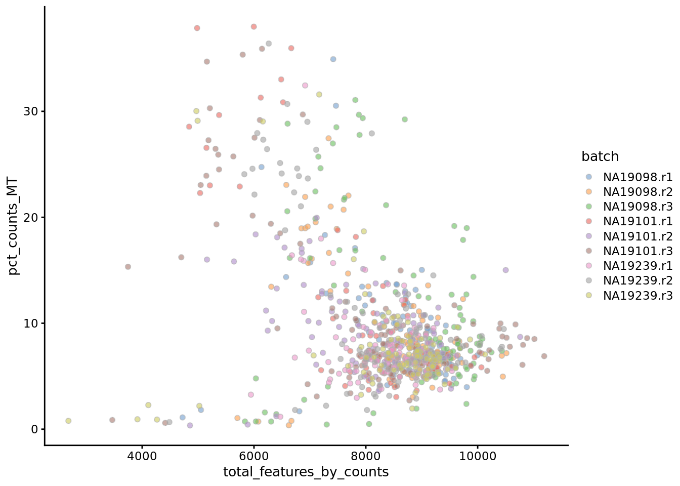
Figure 6.9: Percentage of counts in MT genes
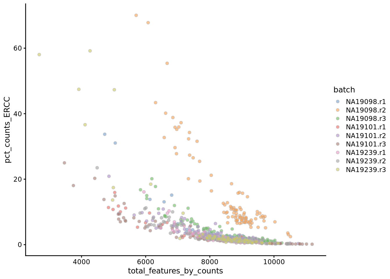
Figure 6.10: Percentage of counts in ERCCs
## filter_by_ERCC
## FALSE  TRUE
## 103 761## filter_by_MT
## FALSE TRUE
## 18 846reads$use <- (
# sufficient features (genes)
filter_by_expr_features &
# sufficient molecules counted
filter_by_total_counts &
# sufficient endogenous RNA
filter_by_ERCC &
# remove cells with unusual number of reads in MT genes
filter_by_MT
)##
## FALSE TRUE
## 258 606## [1] "PCA_coldata"##
## FALSE TRUE
## 753 111plotReducedDim(
reads,
use_dimred = "PCA_coldata",
size_by = "total_features_by_counts",
shape_by = "use",
colour_by = "outlier"
)
##
## Attaching package: 'limma'
## The following object is masked from 'package:scater':
##
## plotMDS## The following object is masked from 'package:BiocGenerics':
##
## plotMAauto <- colnames(reads)[reads$outlier]
man <- colnames(reads)[!reads$use]
venn.diag <- vennCounts(
cbind(colnames(reads) %in% auto,
colnames(reads) %in% man)
)
vennDiagram(
venn.diag,
names = c("Automatic", "Manual"),
circle.col = c("blue", "green")
)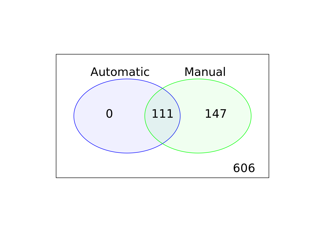
Figure 6.11: Comparison of the default, automatic and manual cell filters
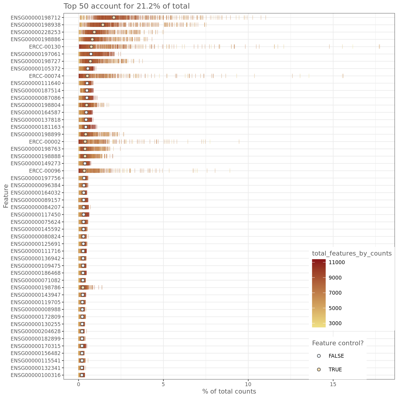
Figure 6.12: Number of total counts consumed by the top 50 expressed genes
keep_feature <- nexprs(
  reads[,colData(reads)$use],
  byrow = TRUE,
  detection_limit = 1
) >= 2
rowData(reads)$use <- keep_feature## keep_feature
## FALSE TRUE
## 2664 16062## [1] 16062 606By comparing Figure 6.5 and Figure 6.11, it is clear that the reads based filtering removed more cells than the UMI based analysis. If you go back and compare the results you should be able to conclude that the ERCC and MT filters are more strict for the reads-based analysis.
## R version 3.6.0 (2019-04-26)
## Platform: x86_64-pc-linux-gnu (64-bit)
## Running under: Ubuntu 18.04.3 LTS
##
## Matrix products: default
## BLAS:   /usr/lib/x86_64-linux-gnu/blas/libblas.so.3.7.1
## LAPACK: /usr/lib/x86_64-linux-gnu/lapack/liblapack.so.3.7.1
##
## locale:
##  [1] LC_CTYPE=en_AU.UTF-8       LC_NUMERIC=C
##  [3] LC_TIME=en_AU.UTF-8        LC_COLLATE=en_AU.UTF-8
##  [5] LC_MONETARY=en_AU.UTF-8    LC_MESSAGES=en_AU.UTF-8
##  [7] LC_PAPER=en_AU.UTF-8       LC_NAME=C
##  [9] LC_ADDRESS=C               LC_TELEPHONE=C
## [11] LC_MEASUREMENT=en_AU.UTF-8 LC_IDENTIFICATION=C
##
## attached base packages:
## [1] parallel  stats4    stats     graphics  grDevices utils     datasets
## [8] methods   base
##
## other attached packages:
##  [1] limma_3.40.6                scater_1.12.2
##  [3] ggplot2_3.2.1               SingleCellExperiment_1.6.0
##  [5] SummarizedExperiment_1.14.1 DelayedArray_0.10.0
##  [7] BiocParallel_1.18.1         matrixStats_0.55.0
##  [9] Biobase_2.44.0              GenomicRanges_1.36.1
## [11] GenomeInfoDb_1.20.0         IRanges_2.18.3
## [13] S4Vectors_0.22.1            BiocGenerics_0.30.0
##
## loaded via a namespace (and not attached):
##   [1] ggbeeswarm_0.6.0         colorspace_1.4-1
##   [3] mvoutlier_2.0.9          class_7.3-15
##   [5] modeltools_0.2-22        rio_0.5.16
##   [7] mclust_5.4.5             XVector_0.24.0
##   [9] pls_2.7-1                BiocNeighbors_1.2.0
##  [11] cvTools_0.3.2            flexmix_2.3-15
##  [13] mvtnorm_1.0-11           ranger_0.11.2
##  [15] splines_3.6.0            sROC_0.1-2
##  [17] robustbase_0.93-5        knitr_1.25
##  [19] zeallot_0.1.0            robCompositions_2.1.0
##  [21] kernlab_0.9-27           cluster_2.1.0
##  [23] rrcov_1.4-7              compiler_3.6.0
##  [25] backports_1.1.4          assertthat_0.2.1
##  [27] Matrix_1.2-17            lazyeval_0.2.2
##  [29] BiocSingular_1.0.0       htmltools_0.3.6
##  [31] tools_3.6.0              rsvd_1.0.2
##  [33] gtable_0.3.0             glue_1.3.1
##  [35] GenomeInfoDbData_1.2.1   dplyr_0.8.3
##  [37] Rcpp_1.0.2               carData_3.0-2
##  [39] cellranger_1.1.0         zCompositions_1.3.2-1
##  [41] vctrs_0.2.0              sgeostat_1.0-27
##  [43] fpc_2.2-3                DelayedMatrixStats_1.6.1
##  [45] lmtest_0.9-37            xfun_0.9
##  [47] laeken_0.5.0             stringr_1.4.0
##  [49] openxlsx_4.1.0.1         lifecycle_0.1.0
##  [51] irlba_2.3.3              DEoptimR_1.0-8
##  [53] zlibbioc_1.30.0          MASS_7.3-51.1
##  [55] zoo_1.8-6                scales_1.0.0
##  [57] VIM_4.8.0                hms_0.5.1
##  [59] RColorBrewer_1.1-2       yaml_2.2.0
##  [61] curl_4.2                 NADA_1.6-1
##  [63] gridExtra_2.3            reshape_0.8.8
##  [65] stringi_1.4.3            highr_0.8
##  [67] pcaPP_1.9-73             e1071_1.7-2
##  [69] boot_1.3-20              zip_2.0.4
##  [71] truncnorm_1.0-8          rlang_0.4.0
##  [73] pkgconfig_2.0.3          prabclus_2.3-1
##  [75] bitops_1.0-6             evaluate_0.14
##  [77] lattice_0.20-38          purrr_0.3.2
##  [79] labeling_0.3             cowplot_1.0.0
##  [81] tidyselect_0.2.5         GGally_1.4.0
##  [83] plyr_1.8.4               magrittr_1.5
##  [85] bookdown_0.13            R6_2.4.0
##  [87] pillar_1.4.2             haven_2.1.1
##  [89] foreign_0.8-70           withr_2.1.2
##  [91] survival_2.43-3          abind_1.4-5
##  [93] RCurl_1.95-4.12          sp_1.3-1
##  [95] nnet_7.3-12              tibble_2.1.3
##  [97] crayon_1.3.4             car_3.0-3
##  [99] rmarkdown_1.15           viridis_0.5.1
## [101] grid_3.6.0               readxl_1.3.1
## [103] data.table_1.12.2        forcats_0.4.0
## [105] diptest_0.75-7           vcd_1.4-4
## [107] digest_0.6.21            tidyr_1.0.0
## [109] munsell_0.5.0            beeswarm_0.2.3
## [111] viridisLite_0.3.0        vipor_0.4.5
6.6 Data visualization and exploratory data analysis
6.6.1 Introduction
In this chapter we will continue to work with the filtered Tung dataset
produced in the previous chapter. We will explore different ways of visualizing
the data to allow you to asses what happened to the expression matrix after the
quality control step. scater package provides several very useful functions to
simplify visualisation.
One important aspect of single-cell RNA-seq is to control for batch effects. Batch effects are technical artefacts that are added to the samples during handling. For example, if two sets of samples were prepared in different labs or even on different days in the same lab, then we may observe greater similarities between the samples that were handled together. In the worst case scenario, batch effects may be mistaken for true biological variation.
Data visualisation can help to identify batch effects or other unwanted sources
of variation that affect our observed gene expression measurements. The Tung
data allows us to explore these issues in a controlled manner since some of the
salient aspects of how the samples were handled have been recorded. Ideally, we
expect to see batches from the same individual grouping together and distinct
groups corresponding to each individual.
Data visualisation and exploratory data analysis are invaluable for allowing us to get a “feel” for a dataset. This is an area of data analysis that is perhaps more art than science, but is a crucial aspect of single-cell QC and analysis.
6.6.2 PCA plot
The easiest way to overview the data is by transforming it using the principal component analysis and then visualize the first two principal components.
Principal component analysis (PCA) is a statistical procedure that uses a transformation to convert a set of observations into a set of values of linearly uncorrelated variables called principal components (PCs). The number of principal components is less than or equal to the number of original variables.
Mathematically, the PCs correspond to the eigenvectors of the covariance matrix. The eigenvectors are sorted by eigenvalue so that the first principal component accounts for as much of the variability in the data as possible, and each succeeding component in turn has the highest variance possible under the constraint that it is orthogonal to the preceding components (the figure below is taken from here).
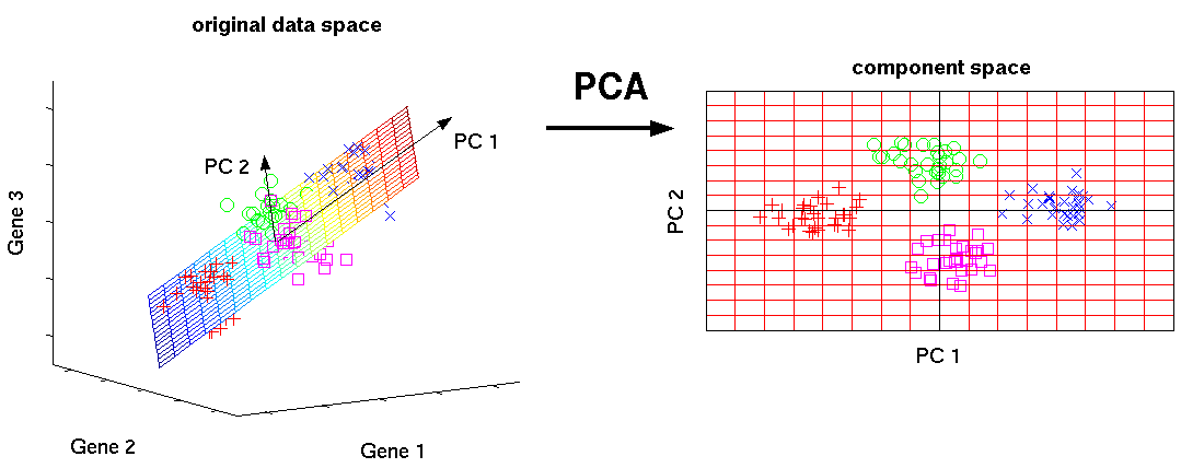
Figure 6.13: Schematic representation of PCA dimensionality reduction
6.6.2.1 Before QC
Without log-transformation:
tmp <- runPCA(
  umi[endog_genes, ],
  exprs_values = "counts"
)
plotPCA(
    tmp,
    colour_by = "batch",
    size_by = "total_features_by_counts",
    shape_by = "individual"
)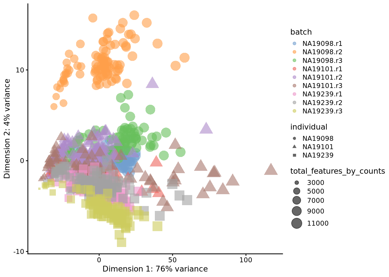
Figure 6.14: PCA plot of the tung data
With log-transformation:
tmp <- runPCA(
  umi[endog_genes, ],
  exprs_values = "logcounts_raw"
)
plotPCA(
    tmp,
    colour_by = "batch",
    size_by = "total_features_by_counts",
    shape_by = "individual"
)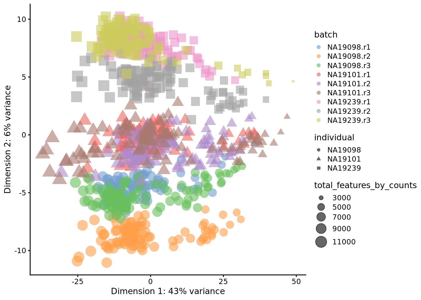
Figure 6.15: PCA plot of the tung data
Clearly log-transformation is benefitial for our data - it reduces the variance on the first principal component and already separates some biological effects. Moreover, it makes the distribution of the expression values more normal. In the following analysis and chapters we will be using log-transformed raw counts by default.
However, note that just a log-transformation is not enough to account for
different technical factors between the cells (e.g. sequencing depth).
Therefore, please do not use logcounts_raw for your downstream analysis,
instead as a minimum suitable data use the logcounts slot of the
SingleCellExperiment object, which not just log-transformed, but also
normalised by library size (e.g. CPM normalisation). In the course we use
logcounts_raw only for demonstration purposes!
6.6.2.2 After QC
tmp <- runPCA(
  umi.qc[endog_genes, ],
  exprs_values = "logcounts_raw"
)
plotPCA(
    tmp,
    colour_by = "batch",
    size_by = "total_features_by_counts",
    shape_by = "individual"
)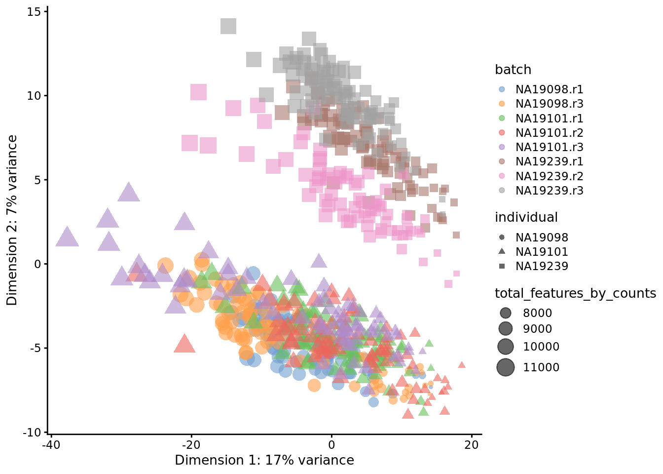
Figure 6.16: PCA plot of the tung data
Comparing Figure 6.15 and Figure 6.16, it is clear that after quality control the NA19098.r2 cells no longer form a group of outliers.
By default only the top 500 most variable genes are used by scater to calculate
the PCA. This can be adjusted by changing the ntop argument.
Exercise 1
How do the PCA plots change if when all 14,066 genes are used? Or when only top 50 genes are used? Why does the fraction of variance accounted for by the first PC change so dramatically?
Hint Use ntop argument of the plotPCA function.
Our answer
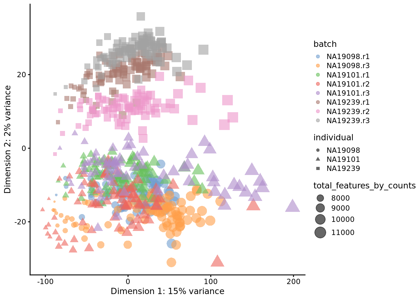
Figure 6.17: PCA plot of the tung data (14214 genes)
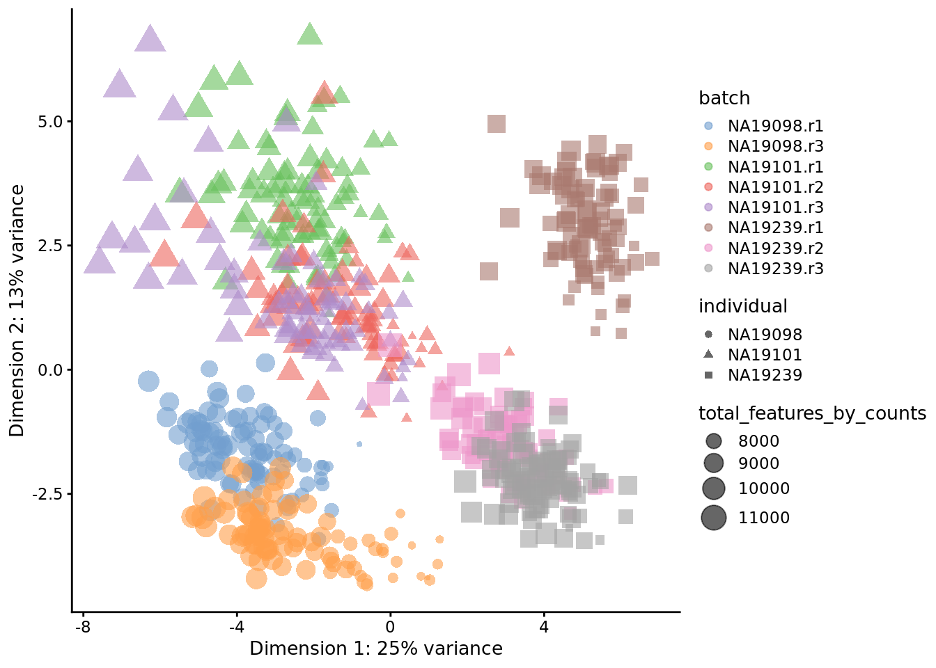
Figure 6.18: PCA plot of the tung data (50 genes)
If your answers are different please compare your code with ours (you need to search for this exercise in the opened file).
6.6.3 tSNE map
An alternative to PCA for visualizing scRNA-seq data is a tSNE plot. tSNE (t-Distributed Stochastic Neighbor Embedding) converts high-dimensional Euclidean distances between datapoints into conditional probabilities that represent similarities, to produce a low-dimensional representation of high-dimensional data that displays large- and local-scale structure in the dataset. Here, we map high dimensional data ( i.e. our 14,214 dimensional expression matrix) to a 2-dimensional space while preserving local distances between cells. tSNE is almost always used to produce a two-dimensional representation of a high-dimensional dataset; it is only rarely used to generate a reduced-dimension space with more than two dimensions and is typically used only for visulisation as opposed being used as a general dimension-reduction method.
Due to the non-linear and stochastic nature of the algorithm, tSNE is more difficult to intuitively interpret than a standard dimensionality reduction method such as PCA. Things to be aware of when using tSNE:
- tSNE has a tendency to (visually) cluster points; as such, it often creates attractive plots of datasets with distinct cell types, but does look as good when there are continuous changes in the cell population.
- The hyperparameters really matter: in particular, changing the perplexity parameter can have a large effect on the visulisation produced. Perplexity is a measure of information, but can loosely be thought of as a tuning parameter that controls the number of nearest neighbous for each datapoint.
- Cluster sizes in a tSNE plot mean nothing.
- Distances between clusters might not mean anything.
- Random noise doesn’t always look random.
- You can see some shapes, sometimes.
For more details about how to use tSNE effectively, see this exellent article.
In contrast with PCA, tSNE is a stochastic algorithm which means running the method multiple times on the same dataset will result in different plots. To ensure reproducibility, we fix the “seed” of the random-number generator in the code below so that we always get the same plot.
6.6.3.1 Before QC
set.seed(123456)
tmp <- runTSNE(
    umi[endog_genes, ],
    exprs_values = "logcounts_raw",
    perplexity = 130
)
plotTSNE(
    tmp,
    colour_by = "batch",
    size_by = "total_features_by_counts",
    shape_by = "individual"
)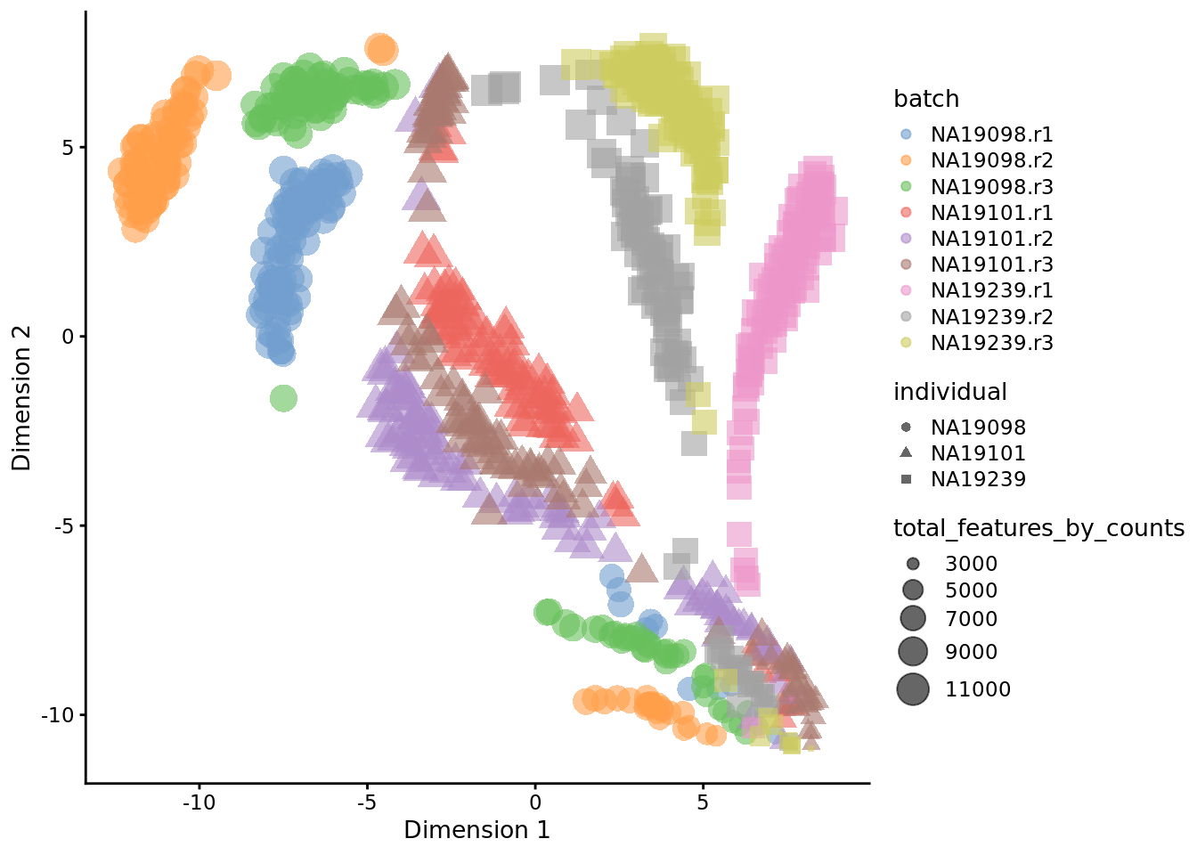
Figure 6.19: tSNE map of the tung data
6.6.3.2 After QC
set.seed(123456)
tmp <- runTSNE(
    umi.qc[endog_genes, ],
    exprs_values = "logcounts_raw",
    perplexity = 130
)
plotTSNE(
    tmp,
    colour_by = "batch",
    size_by = "total_features_by_counts",
    shape_by = "individual"
)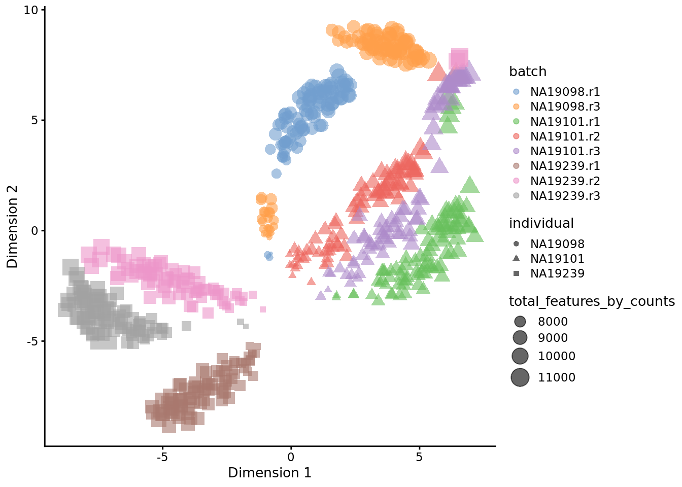
Figure 6.20: tSNE map of the tung data
Interpreting PCA and tSNE plots is often challenging and due to their stochastic and non-linear nature, they are less intuitive. However, in this case it is clear that they provide a similar picture of the data. Comparing Figure 6.19 and 6.20, it is again clear that the samples from NA19098.r2 are no longer outliers after the QC filtering.
Furthermore tSNE requires you to provide a value of perplexity which reflects
the number of neighbours used to build the nearest-neighbour network; a high
value creates a dense network which clumps cells together while a low value
makes the network more sparse allowing groups of cells to separate from each
other. scater uses a default perplexity of the total number of cells divided
by five (rounded down).
You can read more about the pitfalls of using tSNE here.
UMAP (Uniform Manifold Approximation and Projection) is a newer alternative to tSNE which also often creates attractive visualisations of scRNA-seq data with the benefit of being faster than tSNE to compute and is a “true” dimensionality reduction method.
We will look at PCA, tSNE and UMAP plots in subsequent chapters and discuss the topic of dimensionality reduction further in the Latent spaces chapter.
Exercise 2
How do the tSNE plots change when a perplexity of 10 or 200 is used? How does the choice of perplexity affect the interpretation of the results?
Our answer
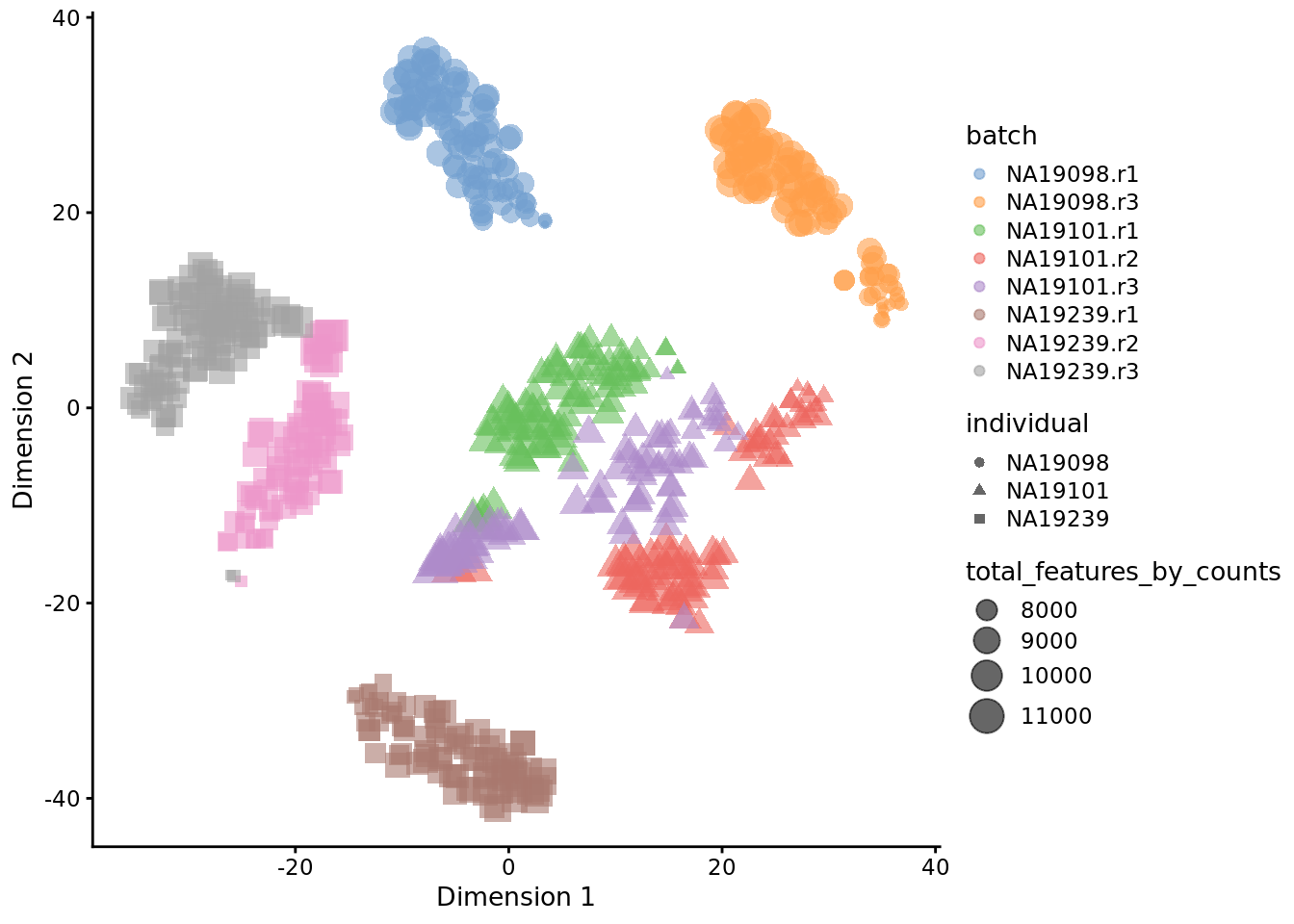
Figure 6.21: tSNE map of the tung data (perplexity = 10)
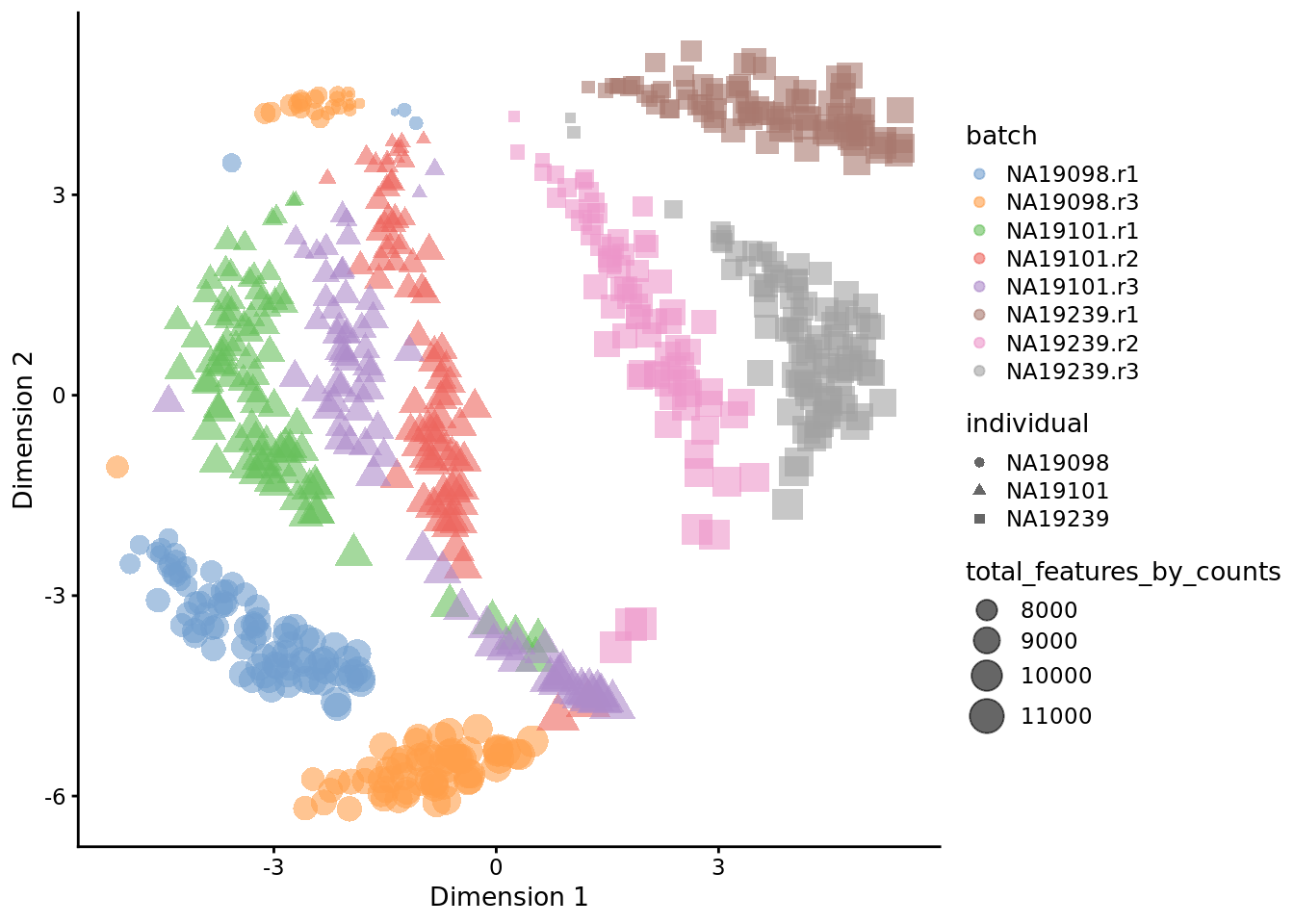
Figure 6.22: tSNE map of the tung data (perplexity = 200)
6.6.4 Big Exercise
Perform the same analysis with read counts of the Blischak data. Use
tung/reads.rds file to load the reads SCE object. Once you have finished
please compare your results to ours (next chapter).
6.6.5 sessionInfo()
## R version 3.6.0 (2019-04-26)
## Platform: x86_64-pc-linux-gnu (64-bit)
## Running under: Ubuntu 18.04.3 LTS
##
## Matrix products: default
## BLAS:   /usr/lib/x86_64-linux-gnu/blas/libblas.so.3.7.1
## LAPACK: /usr/lib/x86_64-linux-gnu/lapack/liblapack.so.3.7.1
##
## locale:
##  [1] LC_CTYPE=en_AU.UTF-8       LC_NUMERIC=C
##  [3] LC_TIME=en_AU.UTF-8        LC_COLLATE=en_AU.UTF-8
##  [5] LC_MONETARY=en_AU.UTF-8    LC_MESSAGES=en_AU.UTF-8
##  [7] LC_PAPER=en_AU.UTF-8       LC_NAME=C
##  [9] LC_ADDRESS=C               LC_TELEPHONE=C
## [11] LC_MEASUREMENT=en_AU.UTF-8 LC_IDENTIFICATION=C
##
## attached base packages:
## [1] parallel  stats4    stats     graphics  grDevices utils     datasets
## [8] methods   base
##
## other attached packages:
##  [1] scater_1.12.2               ggplot2_3.2.1
##  [3] SingleCellExperiment_1.6.0  SummarizedExperiment_1.14.1
##  [5] DelayedArray_0.10.0         BiocParallel_1.18.1
##  [7] matrixStats_0.55.0          Biobase_2.44.0
##  [9] GenomicRanges_1.36.1        GenomeInfoDb_1.20.0
## [11] IRanges_2.18.3              S4Vectors_0.22.1
## [13] BiocGenerics_0.30.0
##
## loaded via a namespace (and not attached):
##  [1] Rcpp_1.0.2               rsvd_1.0.2
##  [3] lattice_0.20-38          assertthat_0.2.1
##  [5] digest_0.6.21            R6_2.4.0
##  [7] evaluate_0.14            highr_0.8
##  [9] pillar_1.4.2             zlibbioc_1.30.0
## [11] rlang_0.4.0              lazyeval_0.2.2
## [13] irlba_2.3.3              Matrix_1.2-17
## [15] rmarkdown_1.15           BiocNeighbors_1.2.0
## [17] labeling_0.3             Rtsne_0.15
## [19] stringr_1.4.0            RCurl_1.95-4.12
## [21] munsell_0.5.0            compiler_3.6.0
## [23] vipor_0.4.5              BiocSingular_1.0.0
## [25] xfun_0.9                 pkgconfig_2.0.3
## [27] ggbeeswarm_0.6.0         htmltools_0.3.6
## [29] tidyselect_0.2.5         tibble_2.1.3
## [31] gridExtra_2.3            GenomeInfoDbData_1.2.1
## [33] bookdown_0.13            viridisLite_0.3.0
## [35] crayon_1.3.4             dplyr_0.8.3
## [37] withr_2.1.2              bitops_1.0-6
## [39] grid_3.6.0               gtable_0.3.0
## [41] magrittr_1.5             scales_1.0.0
## [43] stringi_1.4.3            XVector_0.24.0
## [45] viridis_0.5.1            DelayedMatrixStats_1.6.1
## [47] cowplot_1.0.0            tools_3.6.0
## [49] glue_1.3.1               beeswarm_0.2.3
## [51] purrr_0.3.2              yaml_2.2.0
## [53] colorspace_1.4-1         knitr_1.25
6.7 Exercise: Data visualization (Reads)
library(scater)
options(stringsAsFactors = FALSE)
reads <- readRDS("data/tung/reads.rds")
reads.qc <- reads[rowData(reads)$use, colData(reads)$use]
endog_genes <- !rowData(reads.qc)$is_feature_control
tmp <- runPCA(
reads[endog_genes, ],
exprs_values = "counts"
)
plotPCA(
tmp,
colour_by = "batch",
size_by = "total_features_by_counts",
shape_by = "individual"
)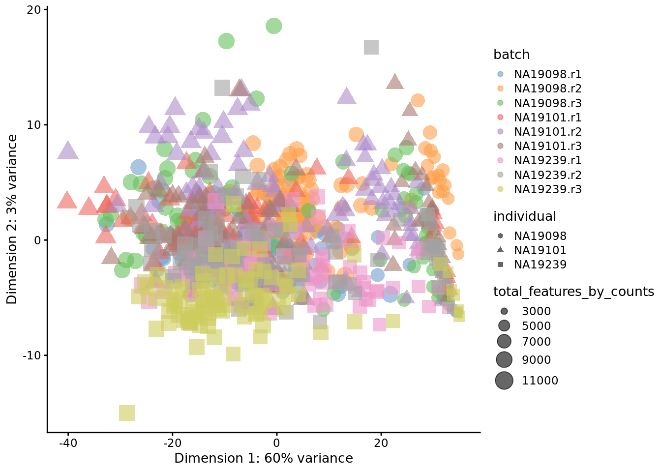
Figure 6.23: PCA plot of the tung data
tmp <- runPCA(
  reads[endog_genes, ],
  exprs_values = "logcounts_raw"
)
plotPCA(
    tmp,
    colour_by = "batch",
    size_by = "total_features_by_counts",
    shape_by = "individual"
)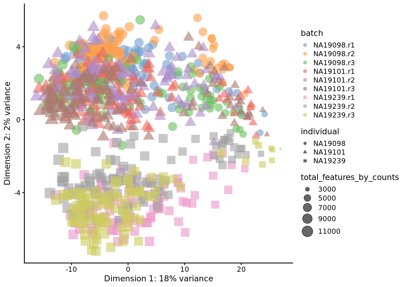
Figure 6.24: PCA plot of the tung data
tmp <- runPCA(
  reads.qc[endog_genes, ],
  exprs_values = "logcounts_raw"
)
plotPCA(
    tmp,
    colour_by = "batch",
    size_by = "total_features_by_counts",
    shape_by = "individual"
)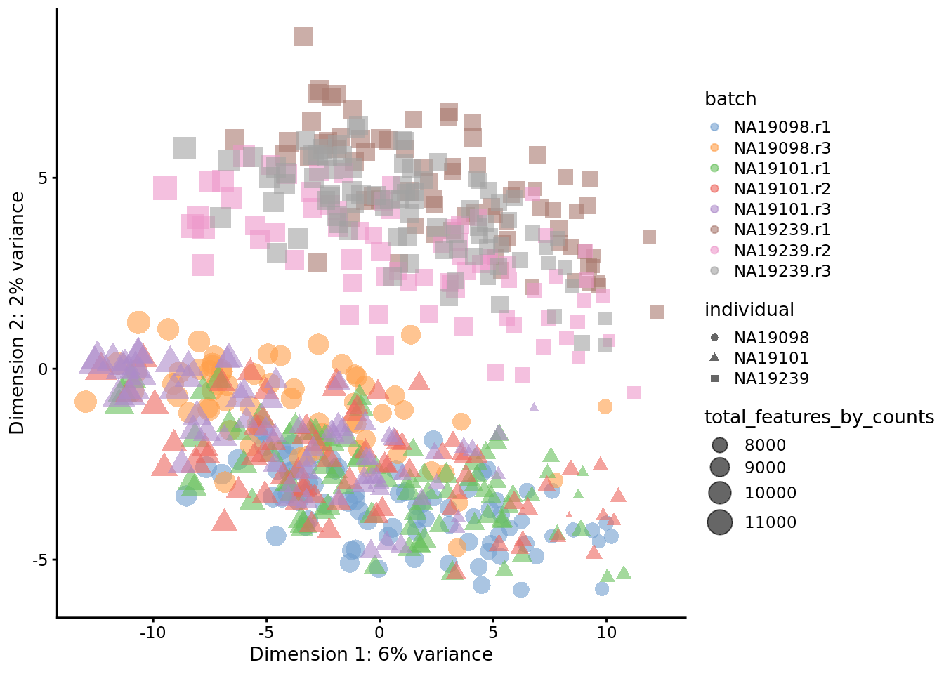
Figure 6.25: PCA plot of the tung data
set.seed(123456)
tmp <- runTSNE(
    reads[endog_genes, ],
    exprs_values = "logcounts_raw",
    perplexity = 130
)
plotTSNE(
    tmp,
    colour_by = "batch",
    size_by = "total_features_by_counts",
    shape_by = "individual"
)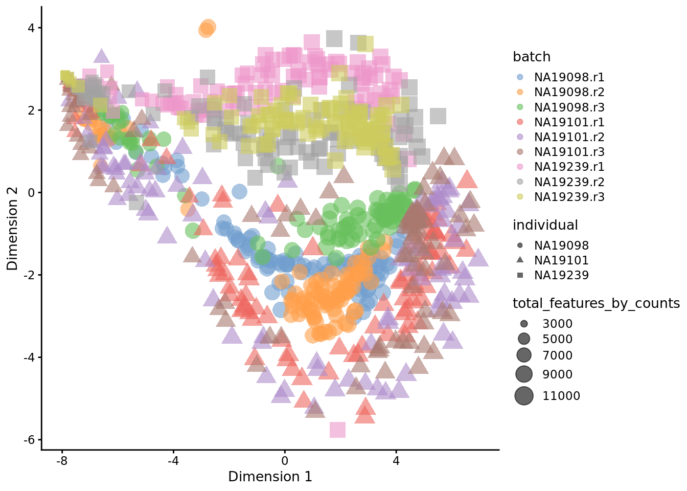
Figure 6.26: tSNE map of the tung data
set.seed(123456)
tmp <- runTSNE(
    reads.qc[endog_genes, ],
    exprs_values = "logcounts_raw",
    perplexity = 130
)
plotTSNE(
    tmp,
    colour_by = "batch",
    size_by = "total_features_by_counts",
    shape_by = "individual"
)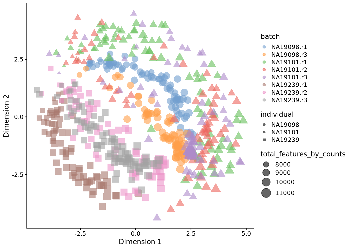
Figure 6.27: tSNE map of the tung data
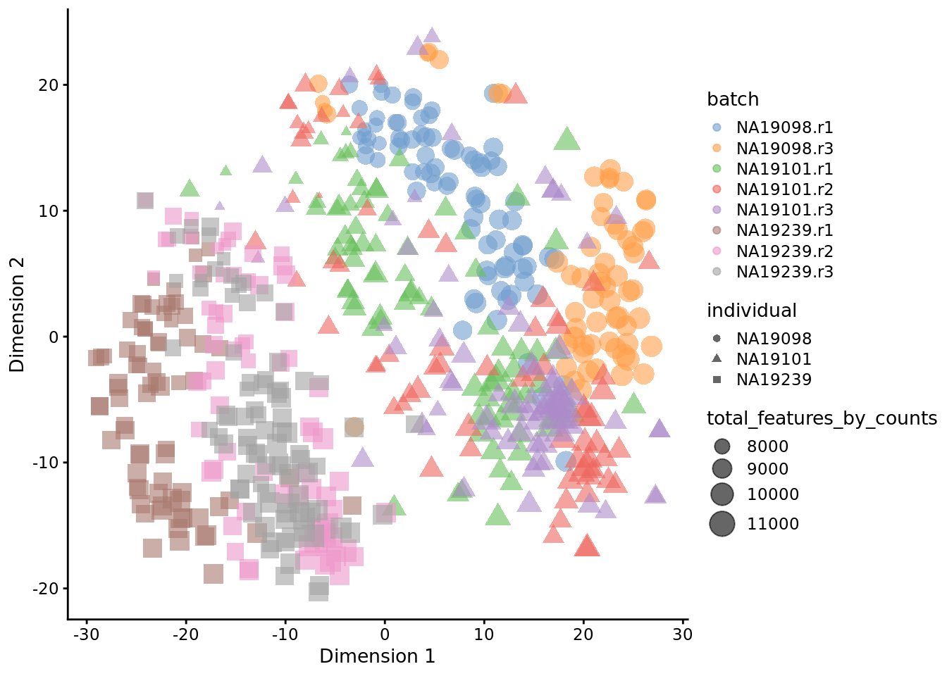
Figure 6.21: tSNE map of the tung data (perplexity = 10)
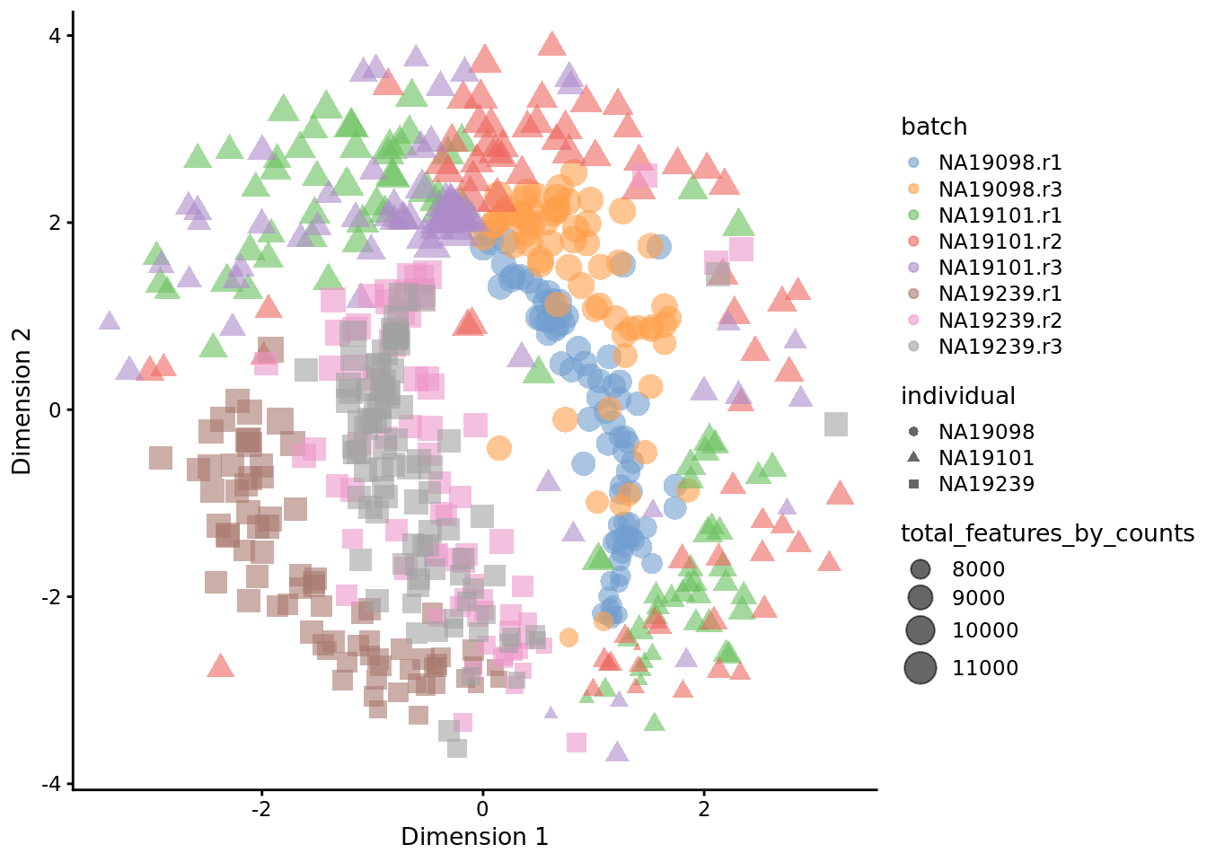
Figure 6.22: tSNE map of the tung data (perplexity = 200)
## R version 3.6.0 (2019-04-26)
## Platform: x86_64-pc-linux-gnu (64-bit)
## Running under: Ubuntu 18.04.3 LTS
##
## Matrix products: default
## BLAS:   /usr/lib/x86_64-linux-gnu/blas/libblas.so.3.7.1
## LAPACK: /usr/lib/x86_64-linux-gnu/lapack/liblapack.so.3.7.1
##
## locale:
##  [1] LC_CTYPE=en_AU.UTF-8       LC_NUMERIC=C
##  [3] LC_TIME=en_AU.UTF-8        LC_COLLATE=en_AU.UTF-8
##  [5] LC_MONETARY=en_AU.UTF-8    LC_MESSAGES=en_AU.UTF-8
##  [7] LC_PAPER=en_AU.UTF-8       LC_NAME=C
##  [9] LC_ADDRESS=C               LC_TELEPHONE=C
## [11] LC_MEASUREMENT=en_AU.UTF-8 LC_IDENTIFICATION=C
##
## attached base packages:
## [1] parallel  stats4    stats     graphics  grDevices utils     datasets
## [8] methods   base
##
## other attached packages:
##  [1] scater_1.12.2               ggplot2_3.2.1
##  [3] SingleCellExperiment_1.6.0  SummarizedExperiment_1.14.1
##  [5] DelayedArray_0.10.0         BiocParallel_1.18.1
##  [7] matrixStats_0.55.0          Biobase_2.44.0
##  [9] GenomicRanges_1.36.1        GenomeInfoDb_1.20.0
## [11] IRanges_2.18.3              S4Vectors_0.22.1
## [13] BiocGenerics_0.30.0
##
## loaded via a namespace (and not attached):
##  [1] Rcpp_1.0.2               rsvd_1.0.2
##  [3] lattice_0.20-38          assertthat_0.2.1
##  [5] digest_0.6.21            R6_2.4.0
##  [7] evaluate_0.14            highr_0.8
##  [9] pillar_1.4.2             zlibbioc_1.30.0
## [11] rlang_0.4.0              lazyeval_0.2.2
## [13] irlba_2.3.3              Matrix_1.2-17
## [15] rmarkdown_1.15           BiocNeighbors_1.2.0
## [17] labeling_0.3             Rtsne_0.15
## [19] stringr_1.4.0            RCurl_1.95-4.12
## [21] munsell_0.5.0            compiler_3.6.0
## [23] vipor_0.4.5              BiocSingular_1.0.0
## [25] xfun_0.9                 pkgconfig_2.0.3
## [27] ggbeeswarm_0.6.0         htmltools_0.3.6
## [29] tidyselect_0.2.5         tibble_2.1.3
## [31] gridExtra_2.3            GenomeInfoDbData_1.2.1
## [33] bookdown_0.13            viridisLite_0.3.0
## [35] crayon_1.3.4             dplyr_0.8.3
## [37] withr_2.1.2              bitops_1.0-6
## [39] grid_3.6.0               gtable_0.3.0
## [41] magrittr_1.5             scales_1.0.0
## [43] stringi_1.4.3            XVector_0.24.0
## [45] viridis_0.5.1            DelayedMatrixStats_1.6.1
## [47] cowplot_1.0.0            tools_3.6.0
## [49] glue_1.3.1               beeswarm_0.2.3
## [51] purrr_0.3.2              yaml_2.2.0
## [53] colorspace_1.4-1         knitr_1.25
References
Bais, Abha S, and Dennis Kostka. 2019. “scds: Computational Annotation of Doublets in Single-Cell RNA Sequencing Data.” Bioinformatics, September. https://doi.org/10.1093/bioinformatics/btz698.
Tung, Po-Yuan, John D. Blischak, Chiaowen Joyce Hsiao, David A. Knowles, Jonathan E. Burnett, Jonathan K. Pritchard, and Yoav Gilad. 2017. “Batch Effects and the Effective Design of Single-Cell Gene Expression Studies.” Sci. Rep. 7 (January). Springer Nature: 39921. https://doi.org/10.1038/srep39921.